Example: 1 Dimensional History Matching
Description
In this Example page we outline a simple but intuitive 1-dimensional example of the history matching process, as described in ThreadGenericHistoryMatching. This will require matching a simple 1-dimensional simulator \(f(x)\) to an observation \(z\), and will involve two waves of refocussing. The notation used is the same as that defined in ThreadGenericHistoryMatching. Here we use the term model synonymously with the term simulator.
Setup
- We have a simple 1D function (a sine wave), which we have used to perform 6 runs.
- The plan is that we will construct an emulator, and use this to evaluate the implausibility function \(I(x)\) over the 1D input space \(\mathcal{X}_0\)
- We will then impose cutoffs to reduce the 1D input space \(\mathcal{X}_0\) down to the non-implausible region denoted \(\mathcal{X}_1\) (see Wave 1 and Figure 1 below).
- Then we perform a second wave of runs (that have inputs belonging to \(\mathcal{X}_1\)) and re-emulate using these new runs.
- The new wave 2 emulator will be more accurate, and hence will change the implausibility function \(I(x)\).
- Imposing the cutoffs on the new implausibility function defines the non-implausible region \(\mathcal{X}_2\), which will be (in this simple example) a good approximation to the set of all acceptable inputs \(\mathcal{X}\) (see Wave 2 and Figure 2 below).
- We do not discuss the emulator construction, except to say here we are using purely a Gaussian process emulator, with no regression terms (this is to allow easier visualisation).
Wave 1
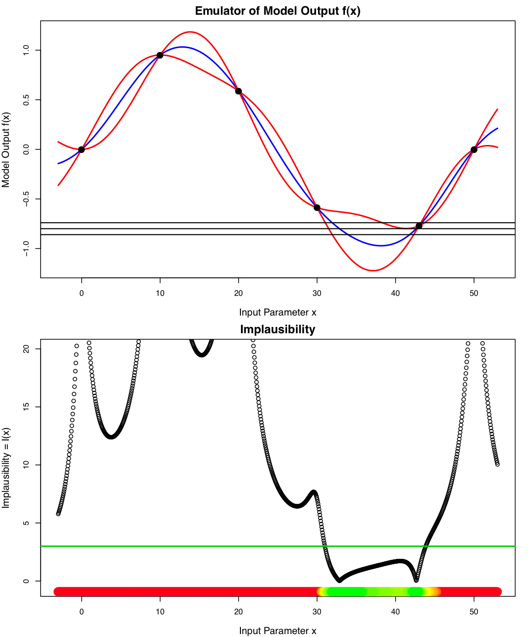
Figure 1: 1D history matching: Wave 1
Figure 1 (top panel) shows:
- The six model runs as black dots (inputs on x-axis, outputs on y-axis).
- The emulator expectation \(\strut{ {\rm E}[f(x)] }\) (blue line).
- Suitable credible intervals (red lines) given by \({\rm E}[f(x)] \pm 3 \sqrt {\rm Var}[f(x)]\).
- The observation \(z=-0.8\) along with \(\pm 3 \sigma\) observational errors, where \(\sigma^2 = {\rm Var}[e] = 0.05^2\) (all given by the 3 horizontal black lines).
Figure 1 (bottom panel) shows:
- The 1D implausibility function \(I(x)\) (black dots).
- The implausibility cutoff level \(c=3\) (thin green line).
- The green colouring on the x axis shows the inputs that belong to the non-implausible region after Wave 1, denoted \(\mathcal{X}_1\)
At this point we perform three more runs within the green region of Figure 1, that is pick new \(x\) values that are members of \(\mathcal{X}_1\) and run the model at these new points.
Wave 2
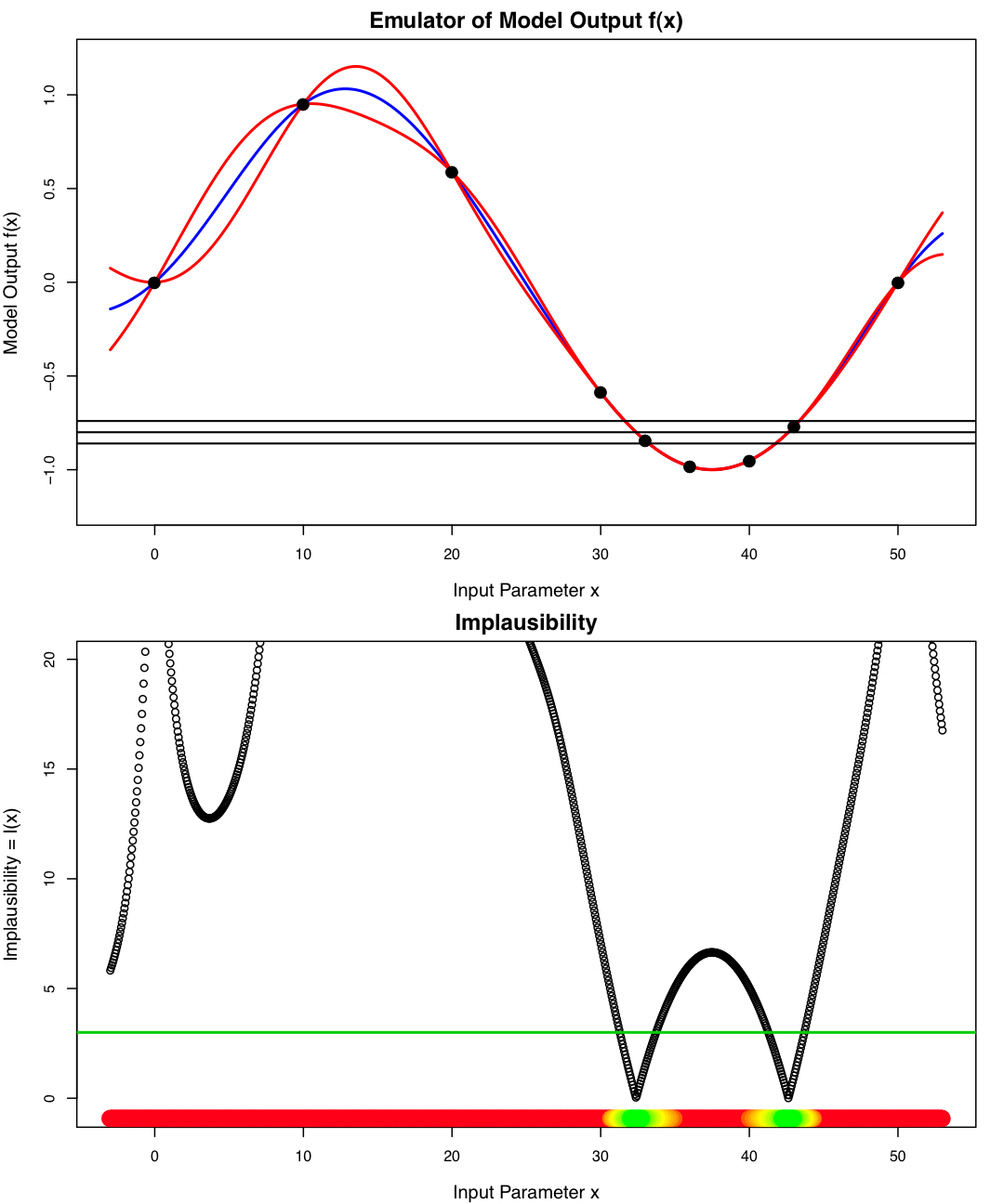
Figure 2: 1D history matching: Wave 2
Figure 2 (top panel) shows how the emulator looks at Wave 2 after the three new runs have been incorporated. Note that:
- The new runs are only in the previous non-implausible region \(\mathcal{X}_1\).
- The emulator is now far more accurate in this \(\mathcal{X}_1\) region (the credible interval given by the red lines is much narrower).
- Further Waves would not be useful as the emulator variance is now far smaller that the observational errors, hence a Wave 3 would not teach us much more about the set of acceptable inputs \(\mathcal{X}\).
Figure 2 (bottom panel) shows the new implausibility measure \(I(x)\) at Wave 2. Note that:
- The implausibility measure \(I(x)\) has increased in certain regions (because we have more information from the 3 new runs).
- The cutoff now defines a smaller non-implausible set \(\mathcal{X}_2\) (given by the green points on the x-axis): this is Refocussing.
- There are now two non-implausible regions of input space remaining: a definite possibility in many applications.
Discussion
The 1-Dimensional example shows the basic history matching process. Note that the model discrepancy was assumed zero for simplicity and to aid visualisation.
When dealing with higher dimensional input spaces, the problem of visualising the results (e.g. the location and shape of the current non-implausible volume \(\mathcal{X}_j\)) becomes important. Various techniques are available including implausibility projections and optical depth plots. See Vernon et. al 2010 for further details.
References
Vernon, I., Goldstein, M., and Bower, R. (2010), “Galaxy Formation: a Bayesian Uncertainty Analysis,” MUCM Technical Report 10/03