Example: A two dimensional emulator with uncertainty and sensitivity analysis
Model (simulator)
In this example we fit a Gaussian process emulator to the surfebm model, using two inputs, the Solar Constant and the Albedo, and one output, the Mean Surface Temperature.
Fitting the emulator
Design
For this example, the input ranges we are interested in are \(\tilde{X}_1 \in [1370,1420]\) for the solar constant and \(\tilde{X}_2 \in [0.2,0.4]\) for the albedo. We obtain our initial design from an \(p=2\)-dimensional optimised Latin Hypercube in \([0,1]\), as described in the procedure page for generating an optimised Latin hypercube design (ProcOptimalLHC). Figure 1 shows the design points mapped in the input space of the model. The \(n=30\) points in \([0,1]\) are arranged in a \((p \times n)\) matrix which we call \(D\).
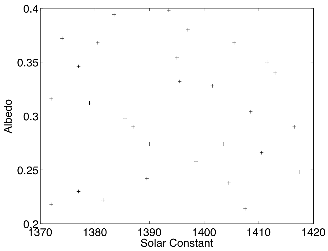
Figure 1: Design points in the simulator’s input space
Having obtained our design points we then run the surfebm model at these points and get the mean surface temperature, which we denote as \(f(D)\).
Gaussian Process setup
As with the one dimensional example, we first set up the Gaussian Process, by selecting a mean and a covariance function. We choose the linear mean function, described in the alternatives page on emulator prior mean function (AltMeanFunction), which is \(h(x) = [1,x]^\textrm{T}\); this is a \((q \times 1)\) vector, with \(q= 1 + p = 3\).
For the covariance function we choose \(\sigma^2c(\cdot,\cdot)\), where the correlation function \(c(\cdot,\cdot)\) has the Gaussian form described in the alternatives page on emulator prior correlation function (AltCorrelationFunction):
where the subscripts \(i\) denote the input.
Estimation of the correlation lengths
The first step in fitting the emulator is to estimate the correlation lengths \(\delta\). We do this by first reparameterising \(\delta\) as \(\tau = 2\ln(\delta)\). This makes the optimisation problem unconstrained, because \(\tau \in [-\infty,\infty]\), whereas \(\delta\in [0,\infty]\). We then find the maximum of the posterior \(\pi^*_{\tau}(\tau)\) assuming a uniform prior on \(\tau\), i.e. \(\pi_{\tau}(\tau) \propto \textrm{const}\). Substitution of \(\delta = \exp(\tau/2)\) in \(\pi^*_{\delta}(\delta)\) from the procedure page on building a Gaussian process emulator for the core problem (ProcBuildCoreGP) yields
with
\(H\) is the \((n \times p)\) matrix \(H=[h(x_1),h(x_2),\cdots,h(x_n)]^\textrm{T}\), with \(x_n\) denoting the \(n\)th design point.
\(A\) is the \(n\times n\) correlation matrix of the design points, with elements \([A]_{i,j} \equiv c(x_i,x_j)\), \(i,j \in \{1,\cdots,n\}\), which after the reparameterisation can be written as
with \(x_{k,i}\) denoting the \(k\)tau` is the correlation matrix \(A\).
Figure 2 shows the log of the posterior \(\pi^*_{\tau}(\tau)\) as a function of \(\tau_1\), which corresponds to the solar constant, and \(\tau_2\), which corresponds to the albedo. The maximum of \(\ln(\pi^*_{\tau}(\tau))\) is found at \(\hat{\tau}=[-1.4001, -4.4864]\). The respective values of \(\delta\) are \(\hat{\delta}=[0.4966, 0.1061]\).
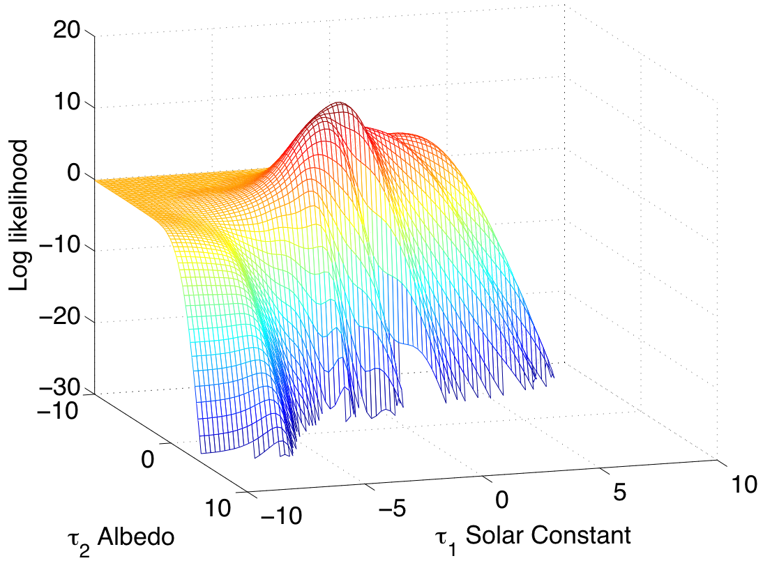
Figure 2: Log posterior \((\ln(\pi^*_{\tau}(\tau)))\) as a function of \(\tau_1\) and \(\tau_2\)
We should mention here that \(\pi^*_{\tau}(\tau)\) can have a complicated structure, exhibiting several local maxima. Therefore, the optimisation algorithm has to be initialised using several starting points so as to find the location of the global maximum, or alternatively, a global optimisation method (e.g. simulated annealing) can be used.
We proceed with our analysis, using for \(\delta\) the estimate
Substitution in the expression for \(\widehat\sigma^2\) yields
Finally, the regression coefficients \(\beta\) are found with the formula
with values \(\hat{\beta}=[33.5758, 4.9908, -39.7233]\)
Validation
After fitting the emulator to the model runs, we need to validate it. We do so by selecting 10 validation points from a Latin hypercube. We call the validation set \(D'\). The validation and the training points are shown in Figure 3.
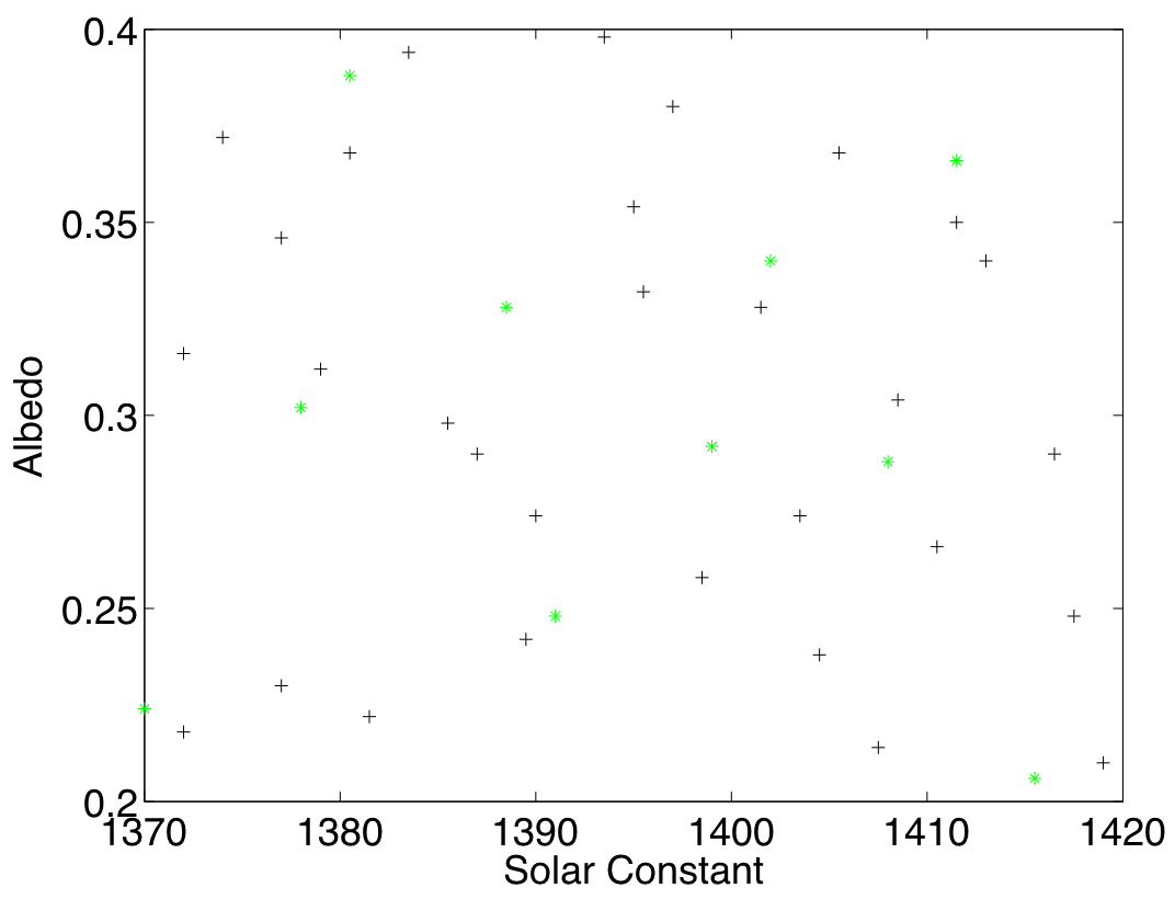
Figure 3: The training (black crosses) and validation points (green stars) in the simulator’s input space
We then run the model at the validation points to obtain its output, which we denote by \(f(D')\). We finally, estimate the posterior mean \(m(D')\) and variance \(u(D',D')\), which are given by the formulae in the procedure page for building a Gaussian process emulator for the core problem (ProcBuildCoreGP)
and
for \(x, x' \in D'\).
The individual standardised errors are then estimated, as it is explained in the procedure page for validating a Gaussian process emulator (ProcValidateCoreGP). As shown in Figure 4 they all lie within 2 standard deviations.
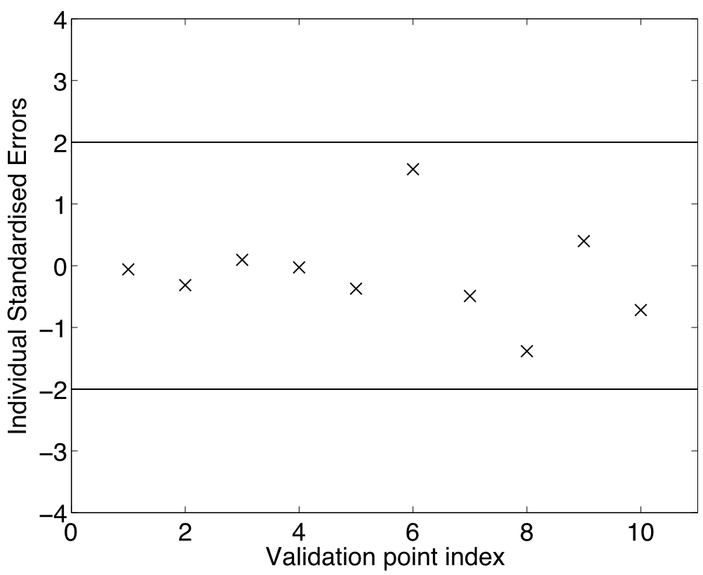
Figure 4: Individual standardised errors
The second validation test we apply is the Mahalanobis distance, also defined in ProcValidateCoreGP. Its value is 8.6027, while its theoretical mean is 10 and its standard deviation is 5.5168. Therefore, the estimated Mahalanobis distance, has a value typical of the reference distribution.
Having passed both tests, the emulator is deemed valid. We therefore rebuild the emulator including the validation data, and use this for the subsequent analysis.
Rebuilding the emulator
The design set for the rebuilt emulator contains the previous training points \(D\) and the validation points \(D'\). That is,
and for simplicity we will denote \(D_{\textrm{new}}\) by \(\strut D\) in the following. Maximising the posterior \(\pi^*_{\tau}(\tau)\), we find \(\hat{\tau} = [-1.2187,-4.6840]\), which corresponds to
and by substitution we find
These parameter values will be used for the uncertainty and sensitivity analysis.
Uncertainty and Sensitivity analysis
Having successfully built the emulator we proceed to perform uncertainty and sensitivity analysis as these are defined in the procedure pages for uncertainty analysis (ProcUAGP) and variance based sensitivity analysis (ProcVarSAGP) using a GP emulator. We start with the uncertainty analysis.
Uncertainty analysis
The primary goal of uncertainty analysis is to quantify the effect of our uncertainty about the input values of the simulator to its output. We denote by \(X\) the model inputs, which are unknown, and we assume that they follow a joint distribution \(\omega(X)\). We wish to know what is the effect of this uncertainty about the inputs \(X\) on the output \(f(X)\). In other words, we seek the mean \(\textrm{E}[f(X)]\) and the variance \(\textrm{Var}[f(X)]\), with respect to the uncertainty distribution \(\omega(X)\).
One method of achieving this would be to use a Monte Carlo method. That would involve drawing samples of \(X\) from \(\omega(X)\) and running the simulator for these input configurations. This method however, requires large computational resources, as we need one simulator run per each Monte Carlo sample. ProcUAGP describes how this can be achieved using the emulator. Specifically, ProcUAGP describes how to calculate the following measures:
- The posterior mean \(\textrm{E}^*[\textrm{E}[f(X)]]\)
- The posterior variance \(\textrm{Var}^*[\textrm{E}[f(X)]]\)
- The posterior mean \(\textrm{E}^*[\textrm{Var}[f(X)]]\)
In the above, \(\textrm{E}[\cdot]\) and \(\textrm{Var}[\cdot]\) are w.r.t. to \(\omega(X)\), and as per usual, \(\textrm{E}^*[\cdot]\) and \(\textrm{Var}^*[\cdot]\) are w.r.t. the emulator.
An interpretation of the above measures could be as follows: the posterior mean \(\textrm{E}^*[\textrm{E}[f(X)]]\) provides us with an estimate of \(\textrm{E}[f(X)]\), which we could also obtain by running the Monte Carlo based method and averaging the model outputs. The posterior variance \(\textrm{Var}^*[\textrm{E}[f(X)]]\) is a measure of the uncertainty about the estimate of \(\textrm{E}[f(X)]\). Finally, the posterior mean \(\textrm{E}^*[\textrm{Var}[f(X)]]\) is an estimate of the variance of \(f(X)\), which is due to \(\omega(X)\) and could be also estimated by finding the variance of the Monte Carlo model outputs.
The input uncertainty distribution
Before starting, we need to define the uncertainty distribution of the inputs, \(\omega(X)\). The definition of this distribution normally requires some interaction with model experts, as discussed in ProcUAGP. For the purposes of our example we will use an independent Gaussian distribution for both inputs. More specifically, for both inputs we will use the distribution
which yields for matrix \(B\)
and
Recall that the above distributions refer to the emulator’s input space, which is the unit interval \([0,1]\). In the simulator’s input space the above distributions are
for the solar constant, and
for the albedo.
We should also mention that the matrix \(C\) is
Also, since we have not used a nugget, we have \(\nu = 0\). Finally, because both \(B\) and \(C\) are diagonal and our regression term has the linear form \(h(x) = [1,x]^{\mathrm{T}}\), we are using the formulae from the special case 2 in ProcUAGP.
Results
We now calculate the three measures, \(\textrm{E}^*[\textrm{E}[f(X)]]\), \(\textrm{Var}^*[\textrm{E}[f(X)]]\) and \(\textrm{E}^*[\textrm{Var}[f(X)]]\). In order to do so we first calculate the integral forms \(U_p,P_p,S_p,Q_p,U,R,T\) from special case 2, and then use them for the calculation of the above measures according to the formulae given at the top of ProcUAGP. The results we got are
The above results say that the mean output of our model, due to the uncertainty in its inputs is \(\sim 16.99\), with a \(95:math:\)pm 1.96sqrt{0.0015} = pm 0.0387`. The variance of the output due to the uncertainty from \(\omega(X)\) is \(\sim 29.96\).
In order to check our results, we run a Monte Carlo simulation, in which 10000 samples were drawn from \(\tilde{X}_1 \sim {\cal N}(1395,50)\) and \(\tilde{X}_2 \sim {\cal N}(0.4,0.0008)\), and the model was run for the ensuing input configurations. The result we got was a mean of 17.16 with a 95% confidence interval of 0.11. The variance of the output was estimated as 29.63. Figure 5 shows the distribution of the Monte Carlo output samples, superimposed on the Gaussian \({\cal N}(\textrm{E}^*[\textrm{E}[f(X)]],\textrm{E}^*[\textrm{Var}[f(X)]])\).
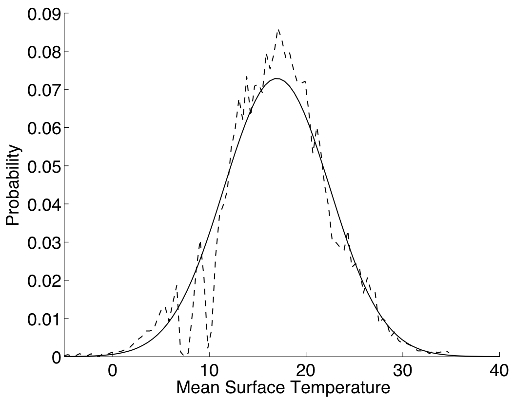
Figure 5: Uncertainty on the output due to \(\omega(X)\), as predicted by the emulator (continuous line) and by using Monte Carlo (dashed line)
When considering the above results, we should also keep in mind the improvement in speed that the Bayesian uncertainty methods achieve. In our implementation, the surfebm model took 0.12 seconds for a single run, and as a result the Monte Carlo simulation took approximately 20 minutes. The emulator based method on the other hand, run almost instantaneously, in less than 0.01 seconds.
Sensitivity analysis
In this section we perform Variance Based Sensitivity Analysis as described in ProcVarSAGP. The main objective of sensitivity analysis is to quantify the effect of our uncertainty about a set of inputs on the output, when the values of the remaining inputs are known. Consequently, it provides a method for assessing the relative importance of the different inputs to the model’s output.
The measures we consider here are the average effect \(\textrm{E}^*[M_w(x_w)]\) and the sensitivity index \(\textrm{E}^*[V_w]\), with \(w\) being the set of indices of the inputs whose value is known, i.e. \(X_w=x_w\). The average effect \(\textrm{E}^*[M_w(x_w)]\) is the difference between the mean of the output when we know the values of the inputs \(X_w\), and the mean of the output when we are uncertain about all the inputs. Therefore, the closer \(\textrm{E}^*[M_w(x_w)]\) is to zero, the smaller the impact the inputs \(X_w\) have on the output.
The sensitivity index \(\textrm{E}^*[V_w]\) quantifies the amount by which the variance of the output will decrease if we were to learn the true value of \(X_w\). Therefore, a large sensitivity index suggests that the inputs \(X_w\) contribute significantly to the output and vice versa. A somewhat subtle point here is that \(\textrm{E}^*[M_w(x_w)]\) is a function of the value that the inputs \(X_w\) take, which we denote by \(x_w\), while \(\textrm{E}^*[V_w]\) is not because the values \(x_w\) are averaged out.
Results
In order to estimate the sensitivity measures, we first need to estimate the integral forms described in special case 2 of ProcVarSAGP, which are \(U_w,P_w,S_w,Q_w,R_w,T_w\) and \(U,P,S,Q,R,T\). Note that \(U,R,T\) are the same as those used in the uncertainty analysis section and we do not need to recalculate them. Similarly, \(\omega(X),B,m,C\) and \(\nu\) are also the same.
Having found the values for the integral forms we can then calculate the two measures using the formulae given at the top of ProcVarSAGP. Figure 6 shows \(\textrm{E}^*[M_1(x_1)]\) and \(\textrm{E}^*[M_2(x_2)]\). We see that \(\textrm{E}^*[M_1(x_1)]\) is significantly closer to zero than \(\textrm{E}^*[M_2(x_2)]\) is. This implies that changing the value of \(X_1\) (solar constant), does not alter significantly the response of the model. The opposite is not true, because \(\textrm{E}^*[M_2(x_2)]\) varies widely as the value of \(X_2\) changes. We could then conclude that the model’s output is significantly more sensitive to the value of the albedo, compared to the value of the solar constant.
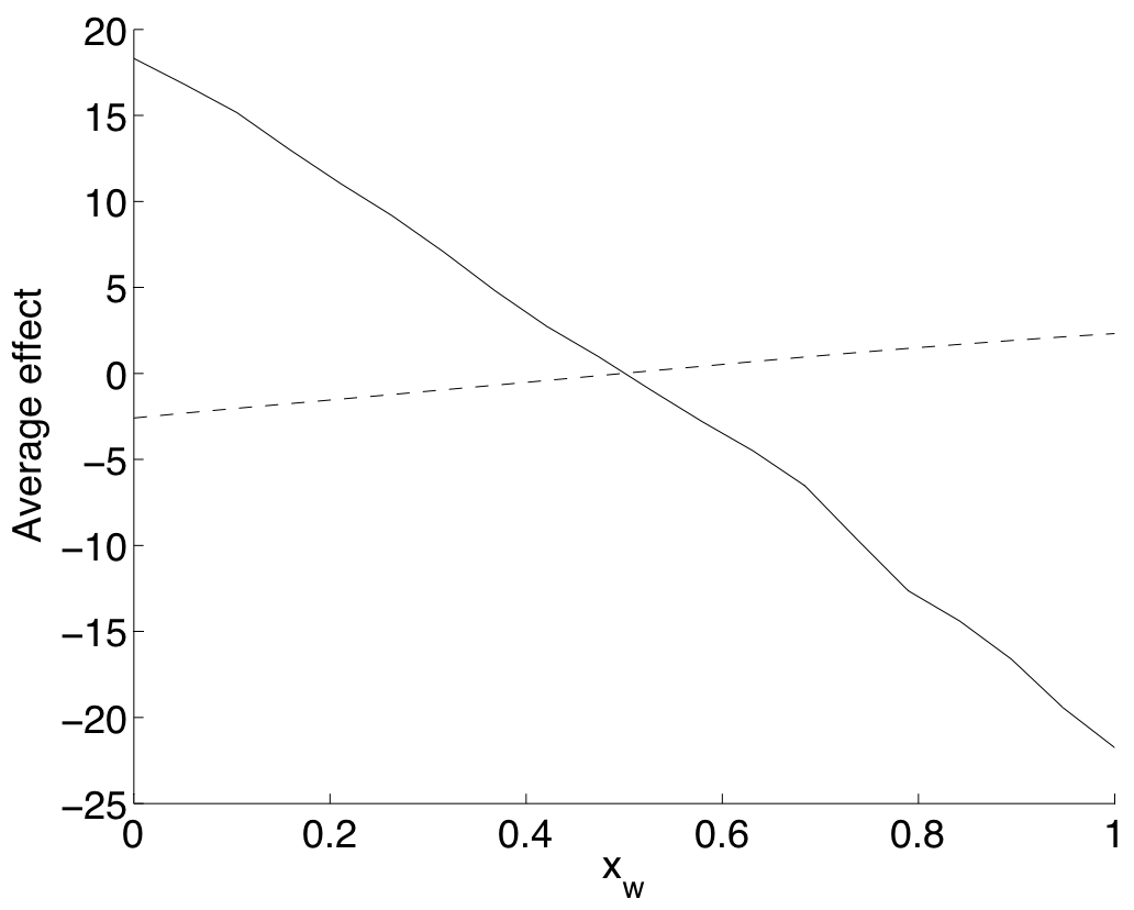
Figure 6: The average effects \(\textrm{E}^*[M_w(x_w)]\) for \(w=1\) (solar constant, dashed line) and \(w=2\) (albedo, continuous line)
The values we calculated for the sensitivity indices are
The results show that when we know the value of \(X_1\), the uncertainty (variance) in the output decreases by 0.54, while when we know the value of \(X_2\) it decreases by 29.40. Recall that the variance of the output when we are uncertain about both \(X_1\) and \(X_2\) was found in the previous section to be 29.96. We can then conclude that if we learn the true value of the albedo, our uncertainty about the model’s output will decrease by approximately 98%, while learning the true value of the solar constant will decrease our uncertainty only by the remaining 2%.
The model
We finally present in Figure 7 the model that we emulated in this example, along with the design points used for building the emulator, shown with black asterisks. Figure 7 indicates that the model’s response depends heavily on the value of the albedo, while the solar constant has a far smaller effect. This intuition is in agreement with the results provided by the sensitivity analysis.
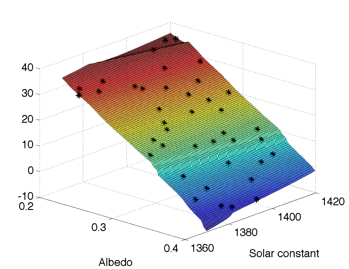
Figure 7: Simulator’s output (mean surface temperature) as a function of the solar constant and the albedo. Black asterisks denote the design points \(D\)
Data
For those wishing to replicate the above results, we provide the values of the design points and the respective model outputs used in this example. The triplets below correspond to \(X_1\) (solar constant), \(X_2\) (albedo) and \(f(X)\) (mean surface temperature).
Original training data
| Solar Constant | 0.86 | 0.27 | 0.57 | 0.5 | 0.14 | 0.23 | 0.39 | 0.93 | 0.98 | 0.54 |
| Albedo | 0.7 | 0.97 | 0.29 | 0.77 | 0.73 | 0.11 | 0.21 | 0.45 | 0.05 | 0.9 |
| Mean Surface Temperature | 11.81 | -4.95 | 25.51 | 5.27 | 4.85 | 30.28 | 27.50 | 20.89 | 34.50 | 0.43 |
| Solar Constant | 0.77 | 0.81 | 0.18 | 0.71 | 0.31 | 0.04 | 0.69 | 0.4 | 0.63 | 0.08 |
| Albedo | 0.52 | 0.33 | 0.56 | 0.84 | 0.49 | 0.09 | 0.19 | 0.37 | 0.64 | 0.86 |
| Mean Surface Temperature | 17.59 | 25.27 | 13.39 | 3.67 | 16.50 | 29.96 | 29.78 | 21.14 | 12.78 | -0.98 |
| Solar Constant | 0.34 | 0.04 | 0.83 | 0.21 | 0.67 | 0.47 | 0.14 | 0.51 | 0.75 | 0.95 |
| Albedo | 0.45 | 0.58 | 0.75 | 0.84 | 0.37 | 0.99 | 0.15 | 0.66 | 0.07 | 0.24 |
| Mean Surface Temperature | 17.99 | 12.11 | 9.10 | 1.03 | 22.71 | -4.61 | 28.33 | 11.60 | 34.10 | 29.28 |
Validation data
| Solar Constant | 0.00 | 0.83 | 0.16 | 0.37 | 0.76 | 0.64 | 0.58 | 0.91 | 0.42 | 0.21 |
| Albedo | 0.12 | 0.83 | 0.51 | 0.64 | 0.44 | 0.70 | 0.46 | 0.03 | 0.24 | 0.94 |
| Mean Surface Temperature | 28.66 | 4.68 | 15.04 | 11.63 | 20.39 | 10.83 | 18.78 | 34.76 | 26.60 | -4.08 |
Recall that the uncertainty and sensitivity analysis was carried out using both data sets above as training data.