Overview

Computer simulations are frequently used in science to understand physical systems, but in practice it can be difficult to understand their limitations and quantify the uncertainty associated with their outputs. This library provides a range of tools to facilitate this process for domain experts that are not necessarily well-versed in uncertainty quantification methods.

This page covers an overview of the workflow. For much more detail, see the Details on the Method section of the introduction, or the Uncertainty Quantification Methods section.

UQ Basics

The UQ workflow here describes the process of understanding a complex simulator. The simulator here is assumed to be a deterministic function mapping multiple inputs to one or more outputs with some general knowledge about the input space. We would like to understand what inputs are reasonable given some observations about the world, and understand how uncertain we are about this knowledge. The inputs may not be something that is physically observable, as they may be standing in for missing physics from the simulator.

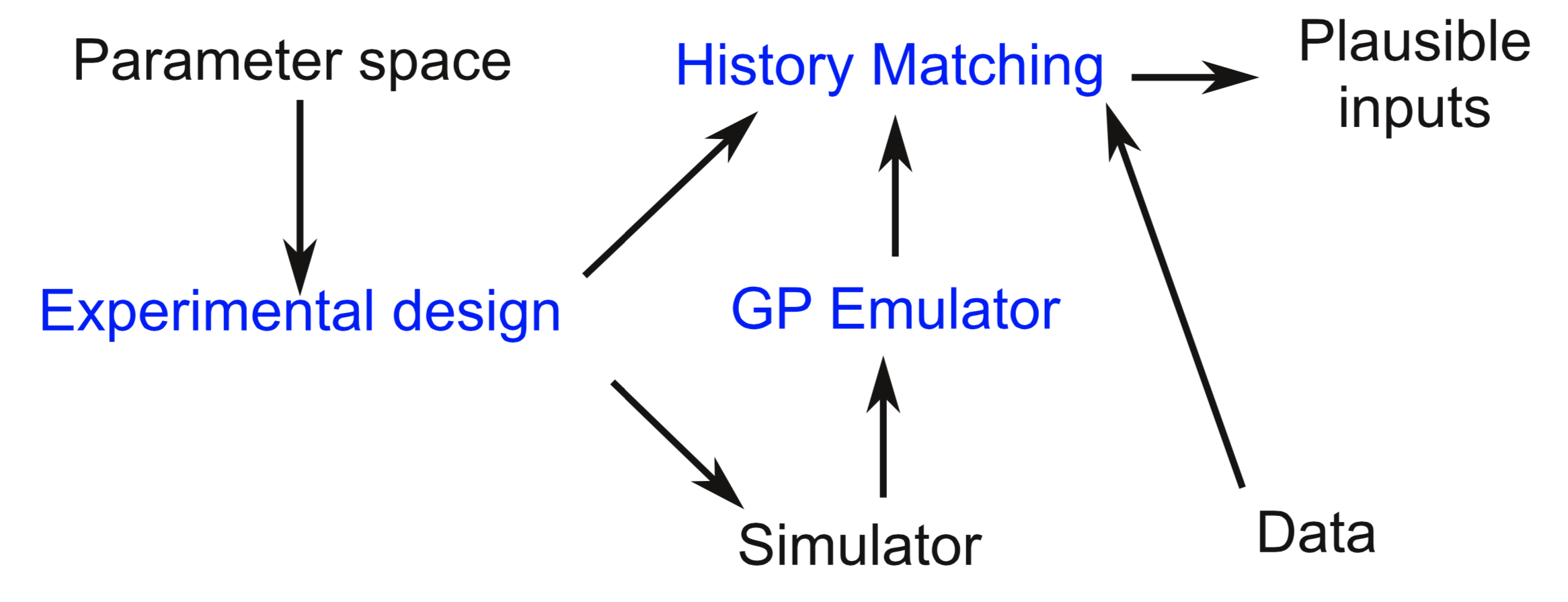
The Uncertainty Quantification workflow. To determine the plausible inputs for a complex simulator given some data and a parameter space, we use an experimental design to sample from the space, run those points through the simulator. To approximate the simulator, we fit a Gaussian Process Emulator to the simulator output. Then, to explore the parameter space, we sample many, many times from the experimental design, query the emulator, and determine the plausible inputs that are consistent with the data using History Matching.

The simulation is assumed to be too expensive to run as many times as needed to explore the entire space. Instead, we will train a surrogate model or emulator model that approximates the simulator and efficiently estimates its value (plus an uncertainty). We will then query that model many times to explore the input space.

Because the simulator is expensive to run, we would like to be judicious about how to sample from the space. This requires designing an experiment to choose the points that are run to fit the surrogate model, referred to as an Experimental Design. Once these points are run, the emulator can be fit and predictions made on arbitrary input points. These predictions are compared to observations for a large number of points to examine the inputs space and see what inputs are reasonable given the observations and what points can be excluded. This is a type of model calibration, and the specific approach we use here is History Matching, which attempts to find the parts of the input space that are plausible given the data and all uncertainties involved in the problem.

Next, we describe the Installation prodecure and provide an example Tutorial to illustrate how this process works.