Tutorial¶

Note: This tutorial requires Scipy version 1.4 or later to run the simulator.

This page includes an end-to-end example of using mogp_emulator to perform model calibration. We define a simulator describing projectile motion with nonlinear drag, and then illustrate how to sample from the simulator, fit a surrogate model, and explore the parameter space using history matching to obtain a plausible subset of the input space.

Projectile Motion with Drag¶

In this example, we will explore projectile motion with drag. A projectile with a mass of 1 kg is fired at an angle of 45 degrees from horizontal and a height of 2 meters. The projectile experiences gravity and drag opposes the motion of the projectile, with a force that is proportional to the squared velocity. For this example, we assume that we do not know the initial velocity or the drag coefficient, but we do know that the projectile travelled 2 km (with a standard deviation measurement error of 20 meters). We would like to determine what inputs could have resulted in this observation.

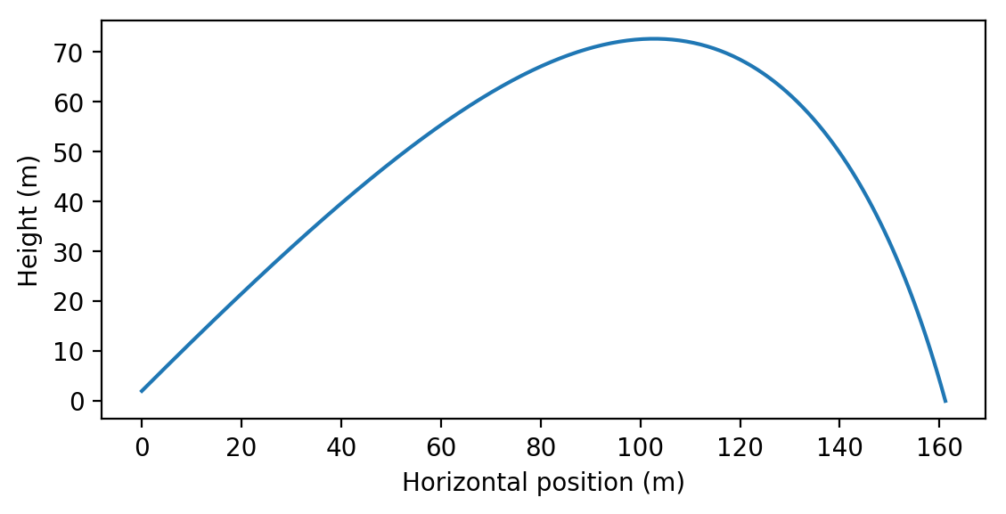
Example simulation of projectile motion with drag for \(C=0.01\) kg/m and \(v_0=100\) m/s computed via numerical integration.

Equations of Motion¶

The equations of motion for the projectile are as follows:

\[\begin{split}m \frac{dv_x}{dt} &= - C v_x \sqrt{v_x^2 + v_y^2} \\ m \frac{dv_y}{dt} &= -g - C v_y \sqrt{v_x^2 + v_y^2} \\ \frac{dx}{dt} &= v_x \\ \frac{dy}{dt} &= v_y\end{split}\]

The initial conditions are

\[\begin{split}v_{x0} &= v_0/\sqrt{2} \\ v_{y0} &= v_0/\sqrt{2} \\ x_{0} &= 0 \\ y_{0} &= h \\\end{split}\]

This can be integrated in time until \(y=0\), and the distance travelled is the value of \(x\) when this occurs.

We include a Python implementation of this model in mogp_emulator/demos/projectile.py. This uses the scipy.integrate function solve_ivp to perform the numerical integration. The RHS derivative is defined in f, and the stopping condition is defined in the event function. The simulator is then defined as a function taking a single input (an array holding the two input parameters of the drag coefficient \(C\) and the initial velocity \(v_0\)) and returning a single value, which is \(x\) at the end of the simulation.

import numpy as np
import scipy
from scipy.integrate import solve_ivp

assert scipy.__version__ >= '1.4', "projectile.py requires scipy version 1.4 or greater"

# Create our simulator, which solves a nonlinear differential equation describing projectile
# motion with drag. A projectile is launched from an initial height of 2 meters at an
# angle of 45 degrees and falls under the influence of gravity and air resistance.
# Drag is proportional to the square of the velocity. We would like to determine the distance
# travelled by the projectile as a function of the drag coefficient and the launch velocity.

# define functions needed for simulator

def f(t, y, c):
    "Compute RHS of system of differential equations, returning vector derivative"

    # check inputs and extract

    assert len(y) == 4
    assert c >= 0.

    vx = y[0]
    vy = y[1]

    # calculate derivatives

    dydt = np.zeros(4)

    dydt[0] = -c*vx*np.sqrt(vx**2 + vy**2)
    dydt[1] = -9.8 - c*vy*np.sqrt(vx**2 + vy**2)
    dydt[2] = vx
    dydt[3] = vy

    return dydt

def event(t, y, c):
    "event to trigger end of integration"

    assert len(y) == 4
    assert c >= 0.

    return y[3]

event.terminal = True

# now can define simulator

def simulator_base(x):
    "simulator to solve ODE system for projectile motion with drag. returns distance projectile travels"

    # unpack values

    assert len(x) == 2
    assert x[1] > 0.

    c = 10.**x[0]
    v0 = x[1]

    # set initial conditions

    y0 = np.zeros(4)

    y0[0] = v0/np.sqrt(2.)
    y0[1] = v0/np.sqrt(2.)
    y0[3] = 2.

    # run simulation

    results = solve_ivp(f, (0., 1.e8), y0, events=event, args = (c,))

    return results

def simulator(x):
    "simulator to solve ODE system for projectile motion with drag. returns distance projectile travels"

    results = simulator_base(x)

    return results.y_events[0][0][2]

Parameter Space¶

We are not sure what values of the parameters to use, so we must pick reasonable ranges. The velocity range might be somewhere in the range of 0-1000 m/s, while the drag coefficient is much more uncertain. For this reason, we use a logarithmic scale to represent the drag coeffient, with values ranging from \(10^{-5}\) to \(10\) kg/m. This will ensure that we sample from a wide range of values to ensure that we understand the effect of this parameter on the simulation.

UQ Implementation¶

As described in Overview, Our analysis consists of three steps:

Drawing parameter values to run our simulator
Fitting a surrogate model to those points
Performing model calibration by sampling many points and comparing to the observations

We will describe each step and provide some code illustrating how the steps are done in mogp_emulator below. The full example is provided in the file mogp_emulator/demos/tutorial.py, and we provide snippets here to illustrate.

Experimental Design¶

For this example, we use a Latin Hypercube Design to sample from the parameter space. Latin Hypercubes attempt to draw from all parts of the distribution, and for small numbers of samples are likely to outperform Monte Carlo sampling.

To define a Latin Hypercube, we must give it the base distributions for all input parameters from which to draw the samples. Because we would like our drag coefficient to be uniformly distributed on a log scale, and the initial velocity to be uniformly distributed on a linear scale, we simply need to provide the upper and lower bounds of the uniform distribution and the Python object will create the distributions for us. If we wanted to use a more complicated distribution, we can pass scipy.stats Point Probability Functions (the inverse of the CDF) when constructing the LatinHypercubeDesign object instead. However, in practice we often do not know much about the parameter distributions, so uniform distributions are fairly common due to their simplicity.

To construct our experimental design and draw samples from it, we do the following:

import numpy as np
from mogp_emulator.demos.projectile import simulator, print_results
import mogp_emulator
import mogp_emulator.validation

lhd = mogp_emulator.LatinHypercubeDesign([(-5., 1.), (0., 1000.)])

n_simulations = 50
simulation_points = lhd.sample(n_simulations)
simulation_output = np.array([simulator(p) for p in simulation_points])

This constructs an instance of LatinHypercubeDesign, and creates the underlying distributions by providing a list of tuples. Each tuple gives the upper and lower bounds on the uniform distribution. Thus, the first tuple determines the drag coefficient (recall that it is on a log scale, so this is defining the distribution on the exponent), and the second determines the initial velocity.

Next, we determine that we want to run 50 simulations. We can get our simulation points by calling the sample method of LatinHypercubeDesign, which is a numpy array of shape (n_simulations, 2). Thus, iterating over the resulting object gives us the parameters for each of our simulations.

We can then simply run our simulation in our Python script. However, for more complicated simulations, we may need to save these values and then submit our jobs to a computer cluster to have the simulations run in a reasonable amount of time.

Gaussian Process Emulator¶

Once we have our simulation points, we fit our surrogate model using the GaussianProcess class. Fitting this model involves giving the GP object our inputs and our targets, and then fitting the parameters of the model using an estimation technique such as Maximum Likelihood Estimation. This is done by passing the GP object to the fit_GP_MAP function, which returns the same GP object but with the parameter values estimated.

gp = mogp_emulator.GaussianProcess(simulation_points, simulation_output, nugget="fit")
gp = mogp_emulator.fit_GP_MAP(gp, n_tries=1)

print("Correlation lengths = {}".format(gp.theta.corr))
print("Sigma = {}".format(np.sqrt(gp.theta.cov)))
print("Nugget = {}".format(np.sqrt(gp.theta.nugget)))

By default, if no priors are specified for the hyperparameters then defaults are chosen. In particular, for correlation lengths, default priors are fit that attempt to put most of the distribution mass in the range spanned by the input data. This tends to stabilize the fitting and improve performance, as fewer iterations are needed to ensure a good fit.

Following fitting, we print out some of the hyperparameters that are estimated. First, we print out the correlation lengths estimated for each of the input parameters. These determine how far we have to move in that coordinate direction to see a significant change in the output. If you run this example, if you get a decent fit you should see correlation lengths of \(\sim 1.3\) and \(\sim 500\) (your values may differ a bit, but note that the fit is not highly sensitive to these values). The overall variation in the function is captured by the variance scale \(\sigma\), which should be around \(\sim 20,000\) for this example.

If your values are very different from these, there is a good chance your fit is not very good (perhaps due to poor sampling). If that is the case, you can run the script again until you get a reasonable fit.

Emulator Validation¶

To show that the emulator is doing a reasonable job, we now cross validate the emulator to compare its predictions with the output from the simulator. This involves drawing additional samples and running the simulations as was done above. However, we also need to predict what the GP thinks the function values are and the uncertainty. This is done with the predict method of GaussianProcess:

n_valid = 10
validation_points = lhd.sample(n_valid)
validation_output = np.array([simulator(p) for p in validation_points])

mean, var, _ = gp.predict(validation_points)

errors, idx = mogp_emulator.validation.standard_errors(gp, validation_points, validation_output)

print_results(validation_points[idx], errors, var[idx])

predictions is an object containing the mean and uncertainty (variance) of the predictions. A GP assumes that the outputs follow a Normal Distribution, so we can perform validation by asking how many of our validation points mean estimates are within 2 standard deviations of the true value by computing the standard errors of the emulator predictions on the validation points. mogp_emulator contains a number of methods of automatically validating an emulator given some validation points, including computing standard errors (see the validation documentation for more details). Usually for this example we would expect about 8/10 to be within 2 standard devations, so not quite as we would expect if it were perfectly recreating the function. However, we will see that this still is good enough in most cases for the task at hand.

History Matching¶

The final step in the analysis is to perform calibration, where we draw a large number of samples from the model input and compare the output of the surrogate model to the observations to determine what inputs are plausible given the data. There are many ways to perform model calibration, but we think that History Matching is a robust technique well-suited for most problems. It has the particular advantage in that even in the situation where the surrogate model is not particularly accurate, the results from History Matching are still valid. This is in contrast to full Bayesian Calibration, where the surrogate model must be accurate over the entire input space to obtain good results.

History matching involves computing an implausibility metric, which determines how likely a particular set of inputs describes the given observations. There are many choices for how to compute this metric, but we default to the simplest version where we compute the number of standard deviations between the surrogate model mean and the observations. The variance is determined by summing the observation error, the surrogate model error, and a final error known as model discrepancy. Model discrepancy is meant to account for the fact that our simulations do not completely describe reality, and is an important consideration in studying most complex physical models. In this example, however, we assume that our model is perfect and the model discrepancy is zero, though we will still consider the other two sources of error.

To compute the implausibility metric, we need to draw a much larger number of samples from the experimental design to ensure that we have good coverage of the input parameter space (it is not uncommon to make millions of predictions when doing history matching in research problems). We draw from our Latin Hypercube Design again, though at this sampling density there is probably not a significant difference between the Latin Hypercube and Monte Carlo sampling (especially in only 2 dimensions). Then, we create a HistoryMatching object and compute which points are “Not Ruled Out Yet” (NROY). This is done as follows:

n_predict = 10000
prediction_points = lhd.sample(n_predict)

hm = mogp_emulator.HistoryMatching(gp=gp, coords=prediction_points, obs=[2000., 400.])

nroy_points = hm.get_NROY()

print("Ruled out {} of {} points".format(n_predict - len(nroy_points), n_predict))

First, we set a large number of samples and draw them from the experimental design object. Then, We construct the HistoryMatching object by giving the fit GP surrogate model (the gp argument), the prediction points to consider (the coords argument), and the observations (the obs argument) as an observed value with an uncertainty (as a variance). The predict method of the GP object is used to make predictions inside the history matching class. With the constructed HistoryMatching object, we can obtain the NROY points by calling the get_NROY method. This returns a list of integer indices that can be used to index into the prediction_points array and learn about the points that are not ruled out by our analysis. We finally print out the fraction of points that were ruled out. In most cases, this should be a large fraction of the space, usually around 98% of the sampled points. Those that are not ruled out are plausible inputs given the data.

We can visualize this quite easily due to the fact that our parameter space is only 2D by making a scatter plot of the NROY points. We also include the sample points used to construct the surrogate model for reference. This plotting command is only executed if matplotlib is installed:

try:
    import matplotlib.pyplot as plt
    makeplots = True
except ImportError:
    makeplots = False

if makeplots:
    plt.figure()
    plt.plot(prediction_points[nroy_points,0], prediction_points[nroy_points,1], "o", label="NROY points")
    plt.plot(simulation_points[:,0], simulation_points[:,1],"o", label="Simulation Points")
    plt.plot(validation_points[:,0], validation_points[:,1],"o", label="Validation Points")
    plt.xlabel("log Drag Coefficient")
    plt.ylabel("Launch velocity (m/s)")
    plt.legend()
    plt.show()

which should make a plot that looks something like this:

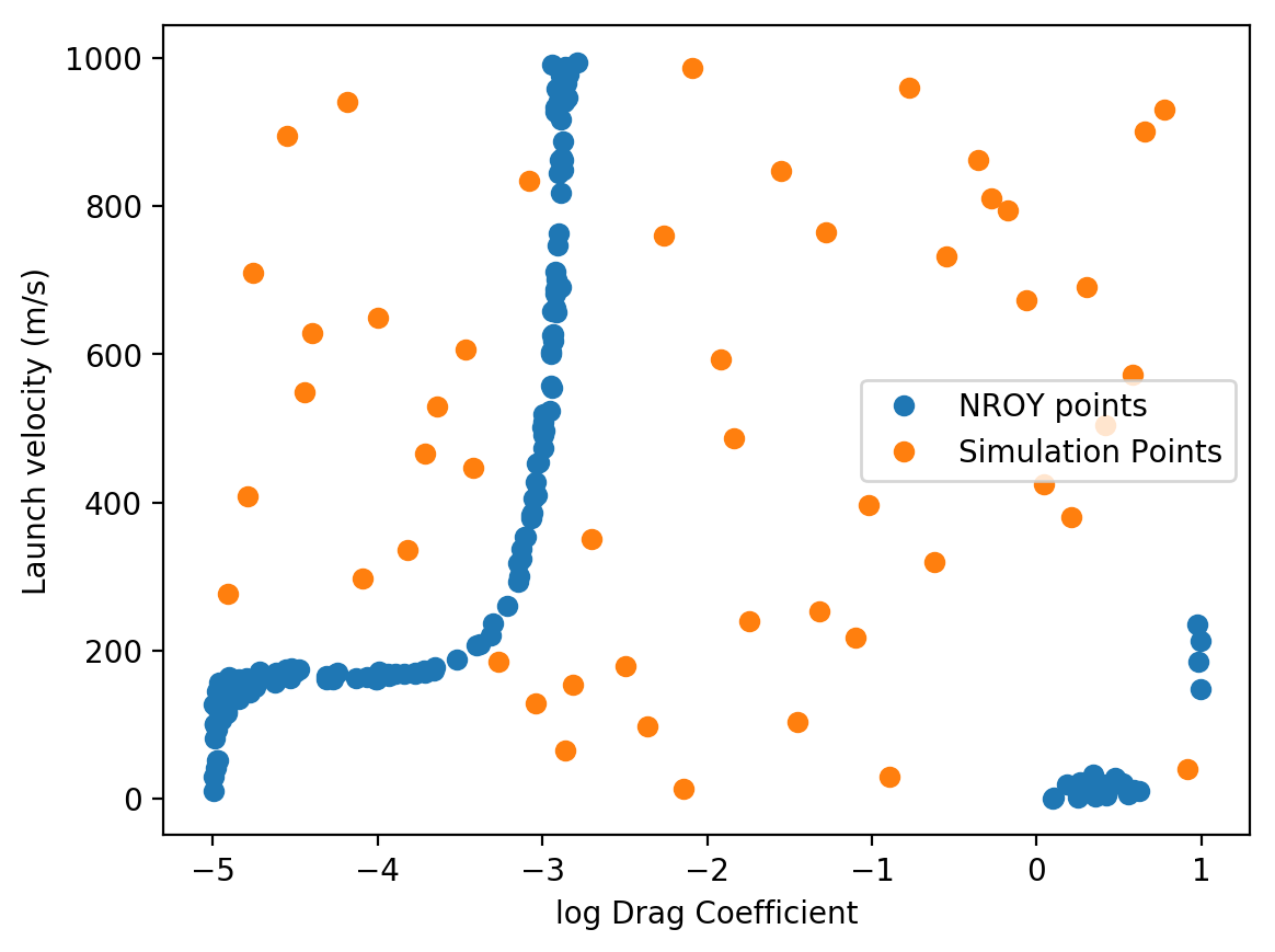
If the original emulator makes accurate predictions, you should get something that looks similar to the above plot. As you can see, most of the space can be ruled out, and only a small fraction of the points remain as plausible options. For launch velocities below around 200 m/s the projectile cannot reach the observed distance regardless of the drag coefficient. Above this value, a narrow range of \((C,v_0)\) pairs are allowed (presumably a line plus some error due to the observation error if our emulator could exactly reproduce the simulator solution). Above a drag coefficient of around \(10^{-3}\) kg/m, none of the launch velocities that we sampled can produce the observations as the drag is presumably too high for the projectile to travel that distance. There are some points at the edges of the simulation that we cannot rule out, though the fact that they occur in gaps in the input simulation sampling suggests that they are likely due to errors in our emulator in those regions.

More Details¶

This simple analysis illustrates the basic approach to running a model calibration example. In practice, this simulator is not particularly expensive to run, and so we could imagine doing this analysis without the surrogate model. However, if the simulation takes even 1 second, drawing the 10,000 samples needed to explore the parameter space would take 3 hours, and a million samples would take nearly 2 weeks. Thus, the surrogate becomes necessary very quickly if we wish to exhaustively explore the input space to the point of being confident in our sampling.

More details about these steps can be found in the Uncertainty Quantification Methods section, or on the following page that goes into more details on the options available in this software library. For more on the specific implementation detials, see the various implementation pages describing the software components.

Table of Contents

Previous topic

Next topic

This Page