Example: Multi-output emulator with separable covariance and dimension reduction
The aim of this example is to illustrate the construction of a multi-output emulator for the chemical reaction simulator described below. The example uses a real model for the decomposition of azoisopropane but does make some simplifying assumptions to enable clearer presentation of the emulation.
Outline
Model (simulator) description
This page provides an example of fitting an emulator to a multi-output simulator. It follows the structure taken in the example for a single output case. The simulator of interest, denoted \(f\), models a chemical reaction in which two initial chemicals react creating new chemical species in the process, while themselves being partially consumed. These new species in turn interact with each other and with the initial reactants to give further species. At the end of the reaction, identified by a stable concentration in all reactants, 39 chemical species can be identified.
The system is deterministic and assumed to be controlled by \(p=12\) inputs: the temperature, the initial concentrations of the 2 reactants and 9 reaction rates controlling the 9 principal reactions. Other reaction rates, for reactions which are present in the system are assumed to be known precisely and are thus fixed - the main reason for doing this is to constrain the number of parameters that need to be estimated in building the emulator. In theory, if this were being done in a real application it would be beneficial to undertake some initial screening to identify the key reactions, if these were not known a priori. The outputs of the simulator are the \(\strut r=39\) final chemical concentrations, measured in log space, which is a common transformation for concentrations which must be constrained to be positive.
Design
We use a space-filling design (maxi-min latin hypercube) over suitable ranges of temperature, initial concentrations of the two species and the 9 key reaction rates. Given the input and output dimensions of the simulator, and therefore emulator, we need a sufficiently large training sample. This is generated by taking a sample of \(n=(r+p)*10=510\) input points within valid ranges. This choice is somewhat arbitrary, but smaller training set sizes were empirically found to produce less reliable emulators. The valid range for each input is taken to be +/-20% of the most likely value specified by the expert. The sample inputs are collected in the design matrix \(\strut D\) and the simulator is evaluated at each point in \(\strut D\), yielding the training outputs \(f(D)\).
Preprocessing
Inputs
The inputs are normalised, so that all input points lie in the unit cube \([0,1]^p\). This is to avoid numerical issues to do with the respective scale of the different inputs (temperatures vary over order 100K while concentrations vary over order 1e-4).
Outputs
Following the procedure page for a principal component transformation of the outputs (ProcOutputsPrincipalComponents), we apply Principal Component Analysis to reduce correlations between outputs, and reduce the dimension of the output domain. However here the aim of using principal components analysis is somewhat different from the reason described in ProcOutputsPrincipalComponents. In ProcOutputsPrincipalComponents the aim is the produce a set of outputs that are as uncorrelated as possible so that each output can be modelled by a separate emulator, as in the generic thread for combining two or more emulators (ThreadGenericMultipleEmulators). In this example the aim is to reduce the output dimensions that need to be emulated, to simplify the emulation task. It may also be beneficial to render the outputs less correlated, but this is not critical here, since a truly multivariate Gaussian process emulator is used.
We first subtract the mean from the data \(F = f(D) - E[f(D)]\) and compute the covariance matrix of the residuals \(F\). We then compute the eigenvalues and eigenvectors of \(\mathrm{cov}(F)\).
Figure 1 shows the eigen-spectrum of the outputs estimated from the 510 training simulator runs.
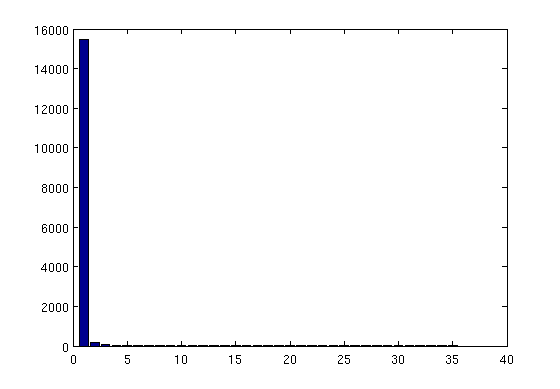
Figure 1: Eigen-values of the principal components on the simulator outputs (based on 510 simulator runs)
The first 10 components (10 largest eigenvalues) explain 99.99% of the variance.
However care must be taken here since the outputs are all very small concentrations expressed in log-space. This means that the lower concentrations are likely to have a larger variance (because of their large negative log-values) than the higher concentrations. Hence, emulating well even the smaller principal components is important. There are several other approaches that could have been taken here, for example it would have been possible to normalise all outputs to lie in \([0,1]^r\), which might make sense if each output was as important as any other. Other approaches to output transformations could be considered, for example changing the transformation, to for example a square root transformation, or a Box-Cox transformation to provide something closer to what is felt to be the important aspect of the simulator to be captured.
In this example we choose to retain \(r^- = 15\) components, rather than the 10 that are apparently sufficient. We then project the training outputs \(f(D)\) onto these first \(r^-\) components, yielding the reduced training outputs \(f^-(D) = f(D) \\times P\), where \(P\) is the \(r\times r^-\) projection matrix made of the first \(r^-\) eigen-vectors.
Note: Projection onto the first 7, 10 and 12 components can be shown to result in poor emulation of the larger concentrations (by retaining 12 principal components, only the largest concentration is incorrectly emulated). All outputs are well emulated with 15 components, as shown below. This is an important point in real applications - think carefully about the outputs you most want to emulate - these might not always appear in the largest eigen-value components.
Complete emulation process
The complete emulation process (including pre-processing) thus comprises of the following steps:
- Choose a design for the training inputs, \(D\), and evaluate the simulator, yielding the training outputs \(f(D)\)
- Normalise the inputs \(x\), yielding \(x^-\)
- Project the training outputs onto the first \(r^-\) principal components, yielding \(f^-(D)\)
- Emulate \(f^- : x^- \rightarrow f^-(D)\)
- Project back onto the \(r\) dimensions of the original output
Any further analysis is performed in projected output space unless specified otherwise. We omit the \(^-\) in the following to keep the notation concise, however we will now work almost exclusively in the projected outputs space.
Gaussian Process emulator setup
Mean function
In setting up the Gaussian process emulator, we need to define the mean and the covariance function. For the mean function, we choose the linear form described in the alternatives page on the emulator prior mean function (AltMeanFunction), with functions \(h(x) = [1,x]^T\) and \(q=1+p = 13\) (\(x\) is 12-dimensional) and regression coefficients \(\beta\). Note the outputs are high dimensional and we assume that each one has its own linear form, meaning there are a lot of regression coefficients \(\beta\).
Covariance function
To emulate the simulator, we use a separable multi-output Gaussian process with a covariance function of the form \(\Sigma \otimes c(.,.)\). The covariance between outputs is assumed to be a general positive semi-definite matrix \(\Sigma\) with elements to be determined below. There is no particular reason to assume a separable form is suitable here, and a later example will show the difference between independent , separable and full covariance emulators. The various options for multivariate emulation are discussed in AltMultipleOutputsApproach.
The correlation function (between inputs) has a Gaussian form:
with \(C\) the diagonal matrix with elements \(C_{ii} = 1/\delta_i^2\) with \(\strut i\) representing each of the \(r\) the (reduced dimension) outputs.
Since the projected training outputs are not a perfect mapping of the original outputs due to the dropped components, we do not want to force the emulator to interpolate these exactly. Thus we add a nugget \(\strut\nu\) to the covariance function, which accounts for the additional uncertainty introduced by the projection as discussed in the alternatives page on emulator prior correlation function (AltCorrelationFunction), and allows the emulator to interpolate the projected training outputs without fitting them exactly. As a side note, adding a nugget also helps to mitigate the computational problems that arise from the use of the Gaussian form in the covariance function. This means that the emulator is no longer an exact interpolation for the simulator, and almost certainly will not reproduce the outputs at training points, although this will be reflected in an appropriate estimate of the emulator uncertainty at these points, which is likely to be very small so long as a sufficient number of components are retained so that the variance of the remaining eigenvalues is very small.
Note that this nugget is added to the covariance between inputs, meaning the total nugget effect is proportional to the between-output covariance \(\Sigma\) and the actual nugget \(\nu\). These are convenient assumptions for computational reasons, which ensure that:
- the covariance function remains separable (which is not the case if the nugget is added to the overall covariance function),
- we can still integrate out \(\Sigma\) (this is made possible by having the nugget proportional to \(\Sigma\)).
In an ideal world we might not want to entangle the nugget and the between outputs variance matrix \(\Sigma\) in this way, however without this modelling choice, that should be validated, we lose the above simplifications which can be very important in high dimensional output settings.
Posterior process
Assuming a weak prior on \((\beta,\Sigma)\), it follows from the procedure page for building a multivariate GP emulator (ProcBuildMultiOutputGP) that we can analytically integrate out \(\beta\) and \(\Sigma\), yielding a posterior t-process. Integrating out these parameters is very advantageous in this setting since these represent a rather large number of parameters which might otherwise need to be optimised or estimated.
Conditional on the covariance function length scales \(\delta\), the mean and covariance functions of the posterior t-process are given by:
where
- \(R(x) = h(x)^{\rm T} - t(x)^{\rm T} A^{-1}H\),
- \(H = h(D)^{\rm T}\),
- _ :math:`widehat{beta}=left( H^{rm T} A^{-1} Hright)^{-1}H^{rm T} A^{-1}
- f(D)`
and
- :math:`widehatSigma = (n-q)^{-1} f(D)^{rm T}left{A^{-1} - A^{-1}
- Hleft( H^{rm T} A^{-1} Hright)^{-1}H^{rm T}A^{-1}right} f(D)`.
Parameter estimation
In order to make predictions, we need to be able to sample from the posterior distribution of \(\delta\), which for a prior \(\pi_\delta(\delta)\) is given by:
A common approximation consists in choosing a single, optimal value for \(\delta\), typically the mode of its posterior distribution (maximum a posteriori). Alternately, if we place an improper uniform prior on \(\delta\), we can set it to the value which maximises the restricted (marginal) likelihood of the data having integrated out \(\beta\) and \(\Sigma\), which is what is done here:
The optimal values of \(\delta\) and \(\nu\) are obtained through minimisation of the negative log of the expression above using a gradient descent method. The optimisation is carried out in log-space to constrain the length scales and nugget variance to remain positive. Thus in this example we fix the nugget and length scales to their most likely values (in a restricted marginal likelihood sense) rather than integrating them out, as might be ideally done - see ProcSimulationBasedInference. This reduces the computational complexity significantly, but could cause some underestimation of emulator uncertainty. Again validation suggests this effect is minimal in this case, but this should always be checked.
Prediction using the emulator
Using the value for \(\delta\) obtained from the previous step, we compute the posterior mean \(m^*(x)\) and variance \(v^*(x)\) at a new input \(x\) as shown above. Further details, such as if we sample from the posterior over \(\delta\) can be found in the procedure page for predicting simulator outputs using a GP emulator (ProcPredictGP).
Projecting back to real space
Since our emulator maps the (normalised) inputs to the reduced output space spanned by the first \(r^-\) principal components, we need to project the \(r^-\)-dimension output of the emulator back onto the full \(r\)-dimension simulator output space. We apply the back-projection matrix \(P^\mathrm{T}\) to the posterior process predictions. That is, at a given input \(x\) with predictive mean and variance \(m^*(x)\) and \(v^*(x)\), we can write:
where \(\xi\) is additional white noise to account for the fact that we have discarded some the principal components when projecting onto the \(r^-\) retained components.
Validation
In order to assess the quality of the emulator, we create a randomly selected test set of \(n' = 300\) inputs \(D'\), at which we compute the emulator’s response. We also compute the true simulator’s response and compare the emulator and the simulator using the diagnostic tools detailed in the procedure page on validating a Gaussian process emulator (ProcValidateCoreGP).
Validation in original (log concentration) space
Figure 2 shows the (marginal) standardised errors at each test point \(x'\) (in no particular order) for the first 16 outputs. The standardised error is the error between the predictive mean \(m(x')\) of the emulator and the true output \(f(x')\), weighted by the predictive variance \(v(x', x')\). Red lines indicate the +/-2 standard deviation intervals. The emulator does a good job (from a statistical point of view) as shown by the appropriate number of errors falling outside the +/-2 standard deviation interval, although there does appear to be something of a bias toward lower valued residuals, which we believe is related to the use of the log transform for very low concentrations.
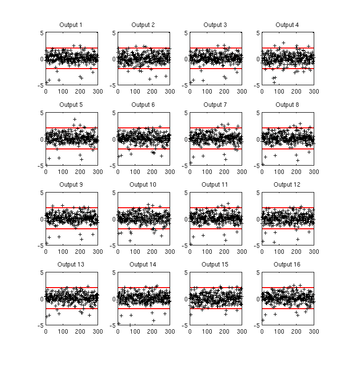
Figure 2: Standardised errors for the 300 test points
In high dimension, visualising marginalised, standardised errors plots quickly becomes impractical. Figure 3 attempts to give a summary of the marginal distribution of the error for all 39 outputs. For each output, we compute a histogram of absolute standardised errors with bin size of 1 standard deviation. We then normalise and plot the histogram as a percentage. For instance, about 50% of the errors fall within 1 standard deviation and about 90% within 2 standard deviations. This confirms that the emulator is correctly representing the uncertainty in the prediction, but these plots are sensitive to small sample errors above 2 standard deviations, and for many outputs the emulator seems somewhat overconfident, which might be due to the fact that the length scale and nugget hyperparameters are not integrated out, but optimised and treated as known.
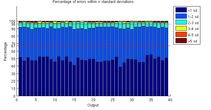
Figure 3: Marginal distribution of absolute errors (percentages, bin size = 1 standard deviation)
Further diagnostics include the Root Mean Square Error (RMSE) and Mahalanobis distance, values for which are provided in Table 1. The RMSE is a measure of the error at each test point and tells us, irrespective of the uncertainty, how close the emulator’s response is to the simulator’s. For the current emulator, we obtain a RMSE of 5.4 for an overall process variance (on average, at a point) of 129.4, which indicates a good fit to the test data. This can be seen to relate to the resolution of the prediction - how close it is to the right value, without reference to the predicted uncertainty. Another measure, which takes into account the uncertainty of the emulator, is the Mahalanobis distance, which for a multi-output emulator is given by:
where
- \(\mathrm{vec}\left[\cdot\right]\) is the column-wise “vectorise” operator,
- \(C\) is the \(n'r \times n'r\) covariance matrix between any two points at any two outputs, i.e. \(C = \Sigma \otimes c(D', D')\).
for which the theoretical mean value is the number of test points. The theoretical mean for the Mahalanobis distance is the number of points, times the number of outputs (due to the vectorisation of the error), i.e. \(E[M] = n'r\). We find that \(M(D') = 11,141\) which is very close to the theoretical 11,700 and confirms the emulator is modelling the uncertainty correctly, that is the predictions are statistically reliable.
| RMSE | Process amplitude | Mahalanobis distance | Theoretical mean |
| 5.4 | 129.4 | 11,141 | 300x39 = 11,700 |
Discussion
This example discussed the emulation of a relatively simple chemical model, which is rather fast to evaluate. The model is quite simple, in that the response to most inputs is quite close to linear and there is significant correlation between outputs. Nevertheless it provides a god case study to illustrate some of the issues one must face in building multivariate emulators. These include
- The size of the training set needs to be large enough to identify the parameters in the covariance function (integrating them all out is computationally very expensive), and to reasonably fill the large input space.
- Using a separable model for the covariance produces significant simplifications allowing many parameters to be integrated out and speeding up the estimation of parameters in the emulator greatly. However there is a price, that the outputs necessarily have the same response to the inputs (modelled by the between inputs covariance function) scaled by the between outputs variance matrix \(\Sigma\).
- When using dimension reduction as part of the emulation process, care must be taken in selecting which components to retain, and careful validation is necessary to establish the quality of the emulator.
Overall the example shows that it is possible to emulate effectively in high dimensions, with the above caveats. In many cases consideration should be given as to whether a joint emulation of the outputs is really needed, but this will be addressed in another example later.