Example: A one-input, two-output emulator
Introduction
In this page we present an example of fitting multivariate emulators to a simple ‘toy’ simulator that evaluates a pair of polynomial functions on a one dimensional input space. We fit emulators with four different types of covariance function:
- an independent outputs covariance function;
- a separable covariance function;
- a convolution covariance function;
- a LMC covariance function.
These covariance functions are described in full in the alternatives page AltMultivariateCovarianceStructures.
Simulator description
The simulator we use has \(p=1\) input and \(r=2\) outputs. It is is a ‘toy’ simulator that evaluates a pair of ninth degree polynomial functions over the input space \([0,1]\). Figures 1(a) and 1(b) show the outputs of the simulator plotted against the input.
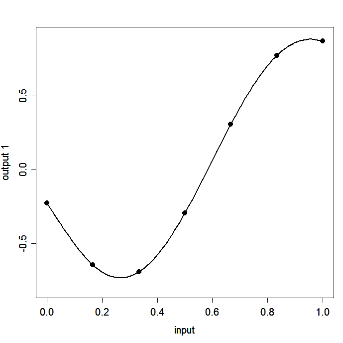
Figure 1(a): Output 1 of the simulator and the 7 design points
Design
Design is the selection of the input points at which the simulator is to be run. There are several design options that can be used, as described in the alternatives page on training sample design for the core problem (AltCoreDesign). For this example, we will simply use a set of \(n=7\) equidistant points on the space of the input variable,
The simulator output at these points is
The true functions computed by the simulator, and the design points, are shown in Figure 1.
Multivariate Gaussian Process setup
In setting up the Gaussian process, we need to define the mean and the covariance function. As mentioned in the introduction we fit four different emulators, each with a different covariance function chosen from the options listed in AltMultivariateCovarianceStructures. They are:
- an independent outputs covariance function with Gaussian form correlation functions;
- a separable covariance function with a Gaussian form correlation function;
- a convolution covariance function with Gaussian form smoothing kernels;
- a LMC covariance function with with Gaussian form basis correlation functions.
We refer to the emulators that result from these four choices as IND, SEP, CONV and LMC respectively.
In all four emulators we assume we have no prior knowledge about how the output will respond to variation in the inputs, so choose a constant mean function as described in AltMeanFunction, which is \(h(x) = 1\) and \(q=1\).
Estimation of the hyperparameters
Each emulator has one or more hyperparameters related to its covariance function, which require a prior specification. The hyperparameters and the priors we use are as follows:
- IND
- Hyperparameters: \(\delta=(\delta_1,\delta_2)\), 2 correlation lengths.
- Prior: \(\pi_\delta(\delta)=\pi_{\delta_1}(\delta_1) \pi_{\delta_2}(\delta_2) \propto \delta_1^{-3} \delta_2^{-3}\). This corresponds to independent noninformative (flat) priors on the inverse squares of the elements of \(\delta\).
- SEP
- Hyperparameter: \(\delta\), the correlation length.
- Prior: \(\pi_\delta(\delta) \propto \delta^{-3}\). This corresponds to a noninformative (flat) prior on the inverse square of \(\delta\).
- CONV
- Hyperparameters: \(\omega=(\delta,\tilde{\Sigma})\), where \(\delta=(\delta_1,\delta_2)\) are 2 correlation lengths for the smoothing kernels.
- Prior: \(\pi_\omega(\omega) \propto \delta_2^{-3} \delta_1^{-3}|\tilde{\Sigma}|^{-3/2}\). This corresponds to independent noninformative priors on \(\tilde{\Sigma}\) and the inverse squares of the elements of \(\delta\).
- LMC
- Hyperparameter: \(\omega=(\tilde{\delta},\Sigma)\), where \(\tilde{\delta}=(\tilde{\delta}_1,\tilde{\delta}_2)\) are 2 basis correlation lengths, and \(\Sigma\), the between outputs covariance function.
- Prior: \(\pi_\omega(\omega) \propto \tilde{\delta}_2^{-3}\tilde{\delta}_1^{-3}|\Sigma|^{-3/2}\). This corresponds to independent noninformative priors on \(\Sigma\) and the inverse squares of the elements of \(\tilde{\delta}\).
We estimate the hyperparameters by maximising the posterior. For IND we take the data from each output \(i=1,2\) in turn and maximise :math:pi^*_{delta_i}(.), the single output GP hyperparameter posterior, as given in ProcBuildCoreGP<ProcBuildCoreGP>. For SEP we maximise :math:pi^*_delta(.) as given in ProcBuildMultiOutputGPSep<ProcBuildMultiOutputGPSep>. For CONV and LMC we maximise :math:pi_omega(.) as given in ProcBuildMultiOutputGP<ProcBuildMultiOutputGP>. The estimates we obtain are as follows:
- IND
- \((\hat{\delta}_1,\hat{\delta}_2)=( 0.6066194, 0.2156990)\)
- SEP
- \(\hat{\delta}=0.1414267\)
- CONV
- \((\hat{\delta}_1,\hat{\delta}_2)= (0.4472136, 0.1777016)\)
- \(\hat{\tilde{\Sigma}}=\left(\begin{array}{cc} 0.4091515 & 0.2576867 \\ 0.2576867 & 0.3039197\end{array} \right)\)
- LMC
- \((\hat{\tilde{\delta}}_1,\hat{\tilde{\delta}}_2)=(0.4472136, 0.2072804)\)
- \(\hat{\Sigma}=\left(\begin{array}{cc} 0.322907165 & 0.006548224 \\ 0.006548224 & 0.254741777 \end{array} \right)\)
Posterior mean and Covariance functions
The expressions for the posterior mean and covariance functions are given in ProcBuildCoreGP for IND , in ProcBuildMultiOutputGPSep for SEP, and in ProcBuildMultiOutputGP for CONV and LMC.
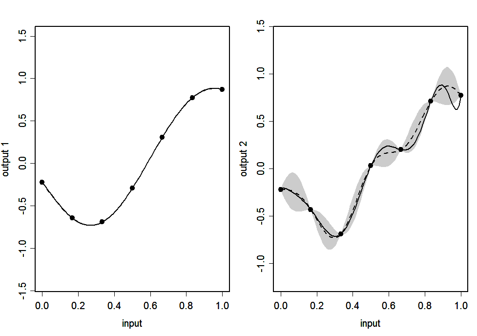
Figure 2(a): IND emulator: Simulator (continuous line), emulator’s mean (dashed line) and 95% posterior intervals (shaded area)
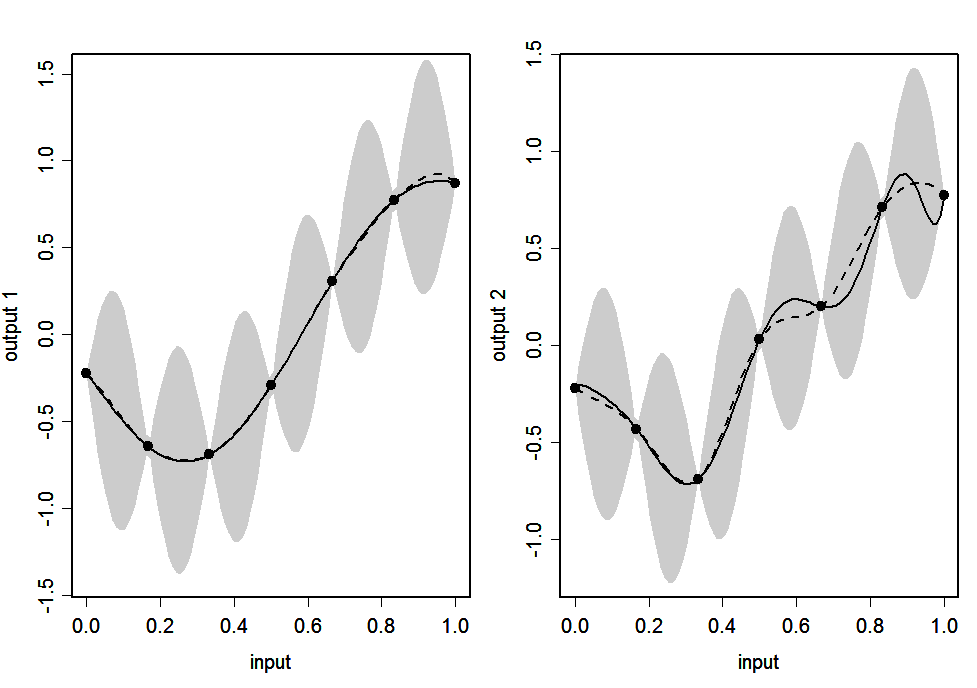
Figure 2(b): SEP emulator: Simulator (continuous line), emulator’s mean (dashed line) and 95% posterior intervals (shaded area)
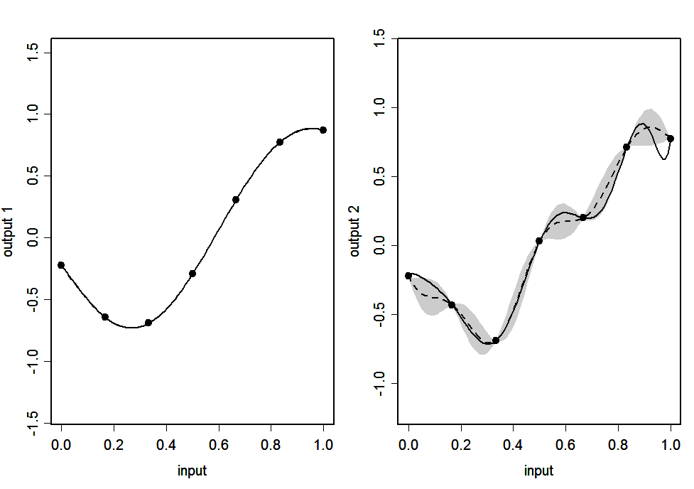
Figure 2(c): CONV emulator: Simulator (continuous line), emulator’s mean (dashed line) and 95% posterior intervals (shaded area)
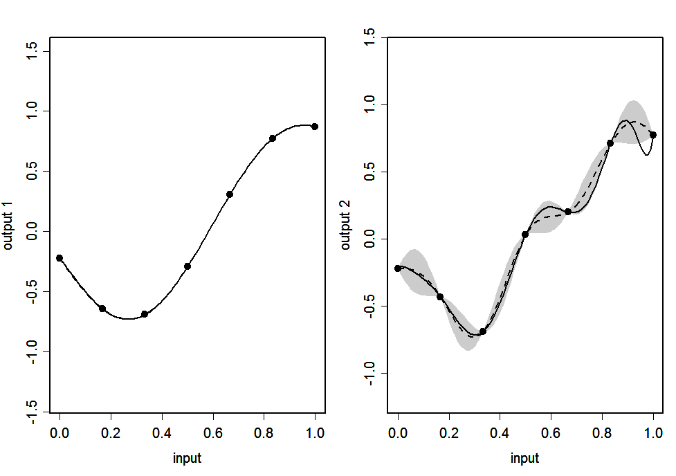
Figure 2(d): LMC emulator: Simulator (continuous line), emulator’s mean (dashed line) and 95% posterior intervals (shaded area)
Figures 2(a)-2(d) show the predictions of the outputs given by the emulators for 100 points uniformly spaced in \([0,1]\). The continuous line is the output of the simulator and the dashed line is the emulator’s posterior mean \(\strut m^*(.)\). The shaded areas represent 2 times the standard deviation of the emulator’s prediction, which is the square root of the diagonal of matrix \(\strut v^*(.,.)\).
We see that, for all four emulators, the posterior mean matches the simulator almost exactly for output 1, but the match is less good for output 2. This is because output 2 has many turning points, and the data miss several extrema, making prediction of these extrema difficult. The main difference between the emulators is in the widths of the posterior 95% interval. For IND, CONV and LMC the interval for output 1 has almost zero width, which is appropriate since there is very little posterior uncertainty about this output, and the interval for output 2 is wide enough to capture the true function in most regions. SEP, on the other hand, has wide intervals for both outputs. This is because both outputs have the same input space correlation function. While the wide interval is appropriate for output 2, it is not appropriate for output 1 as it suggests much more uncertainty about the predictions than necessary.
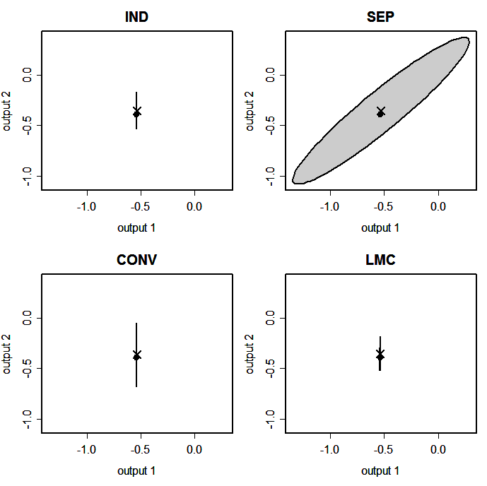
Figure 3(a): Plots of the bivariate output space, showing the simulator output for \(x=0.75\) (black dot), emulator prediction (cross) and 95% posterior region.
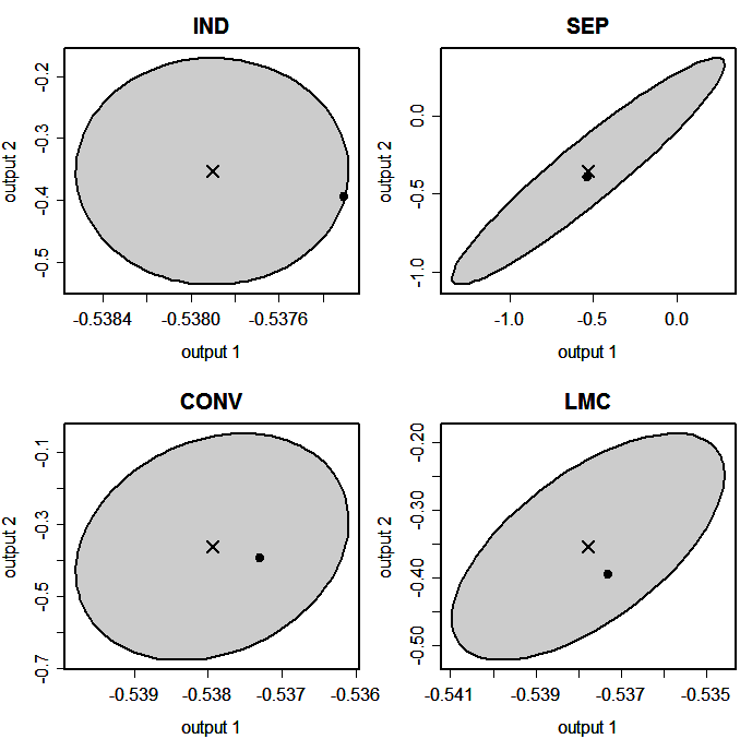
Figure 3(b): The same as Figure 3(a), but with each plot shown on its own axis scales.
Figure 3(a) shows plots of the simulator output and the emulator prediction in the (output 1, output 2)-space at one particular input point, \(x= 0.417\). Also shown is an ellipse that represents the 95% highest probability density posterior region. We see that the 95% ellipses are much smaller for IND, CONV and LMC than for SEP. Figure 3(b) shows the same plots, but with different axis scales, in which we see that the 95% ellipse for IND is symmetric in the coordinate directions, while those for SEP, CONV and LMC are rotated. This shows that the non-independent multivariate emulators have non-zero between-output correlation in their posterior distributions.
Discussion
This example demonstrates some of the features of multivariate emulators with a number of different covariance functions. In summary,
- The independent outputs approach can produce good individual output predictions, and can cope with outputs with different smoothness properties. However, it does not capture the between-outputs correlation, which in this example resulted in a poor representation of joint-output uncertainty.
- The multivariate emulator with a separable covariance function may produce poor results when outputs have different smoothness properties. In this example the problem was mostly with the predictive variance. The feature of having just one input space correlation function for both outputs meant that the posterior uncertainty for at least one output was inappropriate.
- The multivariate emulators with nonseparable covariance functions (the convolution covariance and the LMC covariance) can produce good individual output predictions when outputs have different smoothness properties, and can correctly represent joint-output uncertainty.
This example may suggest that multivariate emulators with nonseparable covariance functions may be the best option in general multi-output problems, since they have the greatest flexibility. However, we must remember this is only a very small-scale example. In larger, more realistic examples, the complexity of nonseparable covariance functions may make them infeasible, due to the large number of hyperparameters that must be estimated. In that case it may come down to a decision between the independent outputs approach (good for individual output predictions) or a multivariate emulator with a separable covariance function (good for representation of joint-output uncertainty).