Discussion: Reification
Description and Background
The most widely used technique for linking a model to reality is that of the Best Input approach, described in the discussion page DiscBestInput. While this simple approach is useful in many applications, we often require more advanced methods to describe adequately the model discrepancy. Here we describe a more careful strategy known as Reification. More details can be found in the reification theory discussion page (DiscReificationTheory). Note that in this page we draw a distinction between the model (the mathematical model of the system) and the simulator (the code that simulates this mathematical model).
In order to think about a more detailed method for specifying model discrepancy, we first discuss three classes of approximations that occur when constructing a simulator. This leads to consideration of improved versions of the model, and we then discuss where in this new framework it would be appropriate to apply a version of the best input approach. This leads us to the reification principle, modelling and application.
Discussion
A More Detailed Specification of Model Discrepancy
When constructing a simulator, there are three classes of approximation that result in differences between the simulator output \(f\) and the real system values \(y\). These are
(a) The limitations of the scientific method chosen. Even if we were able to construct a model which contained all the detailed scientific knowledge we can think about with no known approximations, it would still most likely not be exactly equal to the system \(y\).
(b) Approximations to the scientific account of (a). Often, many theoretical approximations will be made to the model; e.g. mathematical simplifications to the theory, physical processes will be ignored and simplifications to the structure of the model will be made.
(c) Approximations in the implementation of the model. When coding the simulator, often further approximations are introduced which lead to differences between the output of the code and the mathematical model in part (b). A classic example of this is the discretisation of a continuous set of differential equations; e.g. the finite grid in a climate simulator.
These issues and their consequences can be considered at different levels of complexity. A relatively simple way of expressing this situation is by using three unknown functions \(f\), \(f_{\rm theory}\) and \(f^+\) as follows:
- We represent the limit of the scientific method model described in (a) as \(f^+\)
- We represent the current approximate theoretical model described in (b) as \(f_{\rm theory}\)
- We represent the current simulator described in (c) as usual as \(f\)
and we consider how much the current simulator would be changed by moving from (c) to (b) and from (b) to (a). The move from (c) to (b) (i.e. from \(f\) to \(f_{\rm theory}\)) is relatively straightforward to understand and is regularly discussed by modellers (for example, as the error introduced by discretisation). The changes to \(f\) introduced in the move from (b) to (a), that is from \(f_{\rm theory}\) to \(f^+\), is far more complex and requires careful consideration. One practical way of thinking about this is to consider further theoretical improvements to the model in (b). We might represent this as the improved model \(f'_{\rm theory}\) which would lie between (a) and (b). Then we can consider the changes in \(f\) when moving from \(f_{\rm theory}\) to \(f'_{theory}\), and from \(f'_{\rm theory}\) to \(f^+\).
It is now interesting to ask where the best input \(x^+\) and the actual system \(y\) might fit into this structure (see DiscBestInput). It can be shown (see Goldstein, M. and Rougier, J. C. (2009)) that it would place possibly far too strong a constraint on our joint beliefs if we were to insert the same \(x^+\) (with corresponding independent model discrepancies) into all the above models, and that a minimum description allowing maximum flexibility is obtained by inserting \(x^+\) at the top level, into what we define as the Reified model \(f^+\), as is discussed below.
Reified Modelling
Imagine constructing a reified model \(f^+\) which has both (i) sufficiently good physics, and (ii) sufficiently accurate solutions that we have no additional insights as to the nature of any further improvements to \(f^+\). Therefore, the model discrepancy that links \(f^+\) to the real system will be unstructured, for, by definition, there is no improved model that we can think of.
Therefore, we can consistently apply the best input approach to the Reified model; i.e. to \(f^+\) and to \(f^+\) alone, in which case
where \(w\) are any extra model parameters that might be introduced due to any of the considered model improvements, and we take \(\perp\) to mean “independent of” (see DiscReificationTheory for more details).
The Reifying Principle
The Reification approach, which gives a more careful treatment of model discrepancy than the best input approach, is based around the Reification principle, which can be stated as
- The simulator \(f\) is informative for \(y\), because \(f\) is informative for the reified model \(f^+\)
We can represent this in terms of a Bayesian Belief Network, where ‘child’ vertices that are strictly determined by their ‘parents’ are indicated with dashed lines:
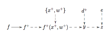
Figure 1: Bayesian Belief Network for the Reification principle.
The reifying principle should be seen as a sensible pragmatic compromise which retains the essential tractability in linking computer evaluations and system values with system behaviour, while removing logical problems in simple treatments of discrepancy, and providing guidance for discrepancy modelling.
If we have several simulators \(f_1, f_2, \ldots, f_r\), then the reifying principle suggests that we combine their information by treating each simulator as informative for the single reified form \(f^+\).
Applying Reification
In order to apply the Reification process, we need to link the current model \(f\), with the Reified model \(f^+\). Often we would employ the use of an emulator to represent \(f\), and from this construct an emulator for \(f^+\). As introduced above, we would possibly consider emulators for intermediate models \(f'\) to resolve specified deficiencies in our modelling. This offers a formal structure to implement the methods suggested in DiscExpertAssessMD for consideration of model discrepancy and helps bridge the gap between \(f\) and \(f^+\). The details of this process, and further discussion of these issues can be found in DiscReificationTheory.
It should be noted that although Reification can sometimes be a complex task, in many cases it is relatively straightforward to implement, especially if the expert does not have detailed ideas about possible improvements to the model. In this case, it can be as simple as inflating the variances of some of the uncertain quantities contained in the emulator for \(f\); see, Goldstein, M. and Rougier, J. C. (2009). It should also be stressed that Reification provides a formally consistent approach to linking families of models to reality, in contrast with the Best Input approach.
Additional Comments
A particular example of Reification is provided by Exchangeable Computer Models: see DiscExchangeableModels for further discussion of this area.
References
Goldstein, M. and Rougier, J. C. (2009), “Reified Bayesian modelling and inference for physical systems (with Discussion)”, Journal of Statistical Planning and Inference, 139, 1221-1239.