Discussion: Reification Theory
Description and Background
Reification is an approach for coherently linking models to reality, which was introduced in the discussion page DiscReification. Here we provide more detail about the various techniques involved in implementing the full Reification process. Readers should be familiar with the basic emulation ideas presented in the core threads ThreadCoreGP and specifically ThreadCoreBL.
Discussion
As covered in DiscReification, the Reification approach centres around the idea of linking the current model \(f\) to a Reified model \(f^+\). The Reified model incorporates all possible improvements to the model that can be currently imagined. The link to reality :math:y is then given by applying the Best Input<DefBestInput> approach (see DiscBestInput) to the Reified model only, giving,
where \(w\) are any extra model parameters that might be introduced due to any of the considered model improvements incorporated by \(f^+\). Hence, this is a more detailed method than the Best Input approach. Here we will describe in more detail how to link a model \(f\) to \(f^+\) either directly (a process referred to as Direct Reification) or via an intermediate model \(f'\) (a process referred to as Structural Reification). This involves the use of emulators to summarise our beliefs about the behaviour of each of the functions \(f\), \(f'\) and \(f^+\). Here \(f'\) may correspond to any of the intermediate models introduced in DiscReification.
Direct Reification
Direct Reification is a relatively straightforward process where we link the current model \(f\) to the Reified model \(f^+\). It should be employed when the expert does not have detailed ideas about specific improvements to the model.
We first represent the model \(f\) using an emulator. As described in detail in ThreadCoreGP and ThreadCoreBL, an emulator is a probabilistic belief specification for a deterministic function. Our emulator for the \(i\) might take the form,
where \(B = \{ \beta_{ij} \}\) are unknown scalars, \(g_{ij}\) are known deterministic functions of the inputs \(x\), and \(u_i(x)\) is a weakly stationary stochastic process.
The Reified model might be a function, not just of the current input parameters \(x\) , but also of new inputs \(w\) which might be included in a future improvement stage. Our simplest emulator for \(f^+\) would then be
where we might model \(B^+ = \{ \beta^+_{ij} \}\) as \(\beta^+_{ij} = c_{ij}\, \beta_{ij} + \nu_{ij}\) for known \(c_{ij}\) and uncertain \(\nu_{ij}\), and correlate \(u_i(x)\) and \(u_i^+(x)\), but leave \(u_i^+(x,w)\) uncorrelated with the other random quantities in the emulator. Essentially this step models \(f^+\) by inflating each of the variances in the current emulator for \(f\), and is often relatively simple. We can represent this structure using the following Bayesian Belief Network, where ‘child’ vertices that are strictly determined by their ‘parents’ are indicated with dashed lines, where \(u^+\) represents \(\{ u^+(x), u^+(x,w) \}\) and \(F\) represents a collection of model runs:
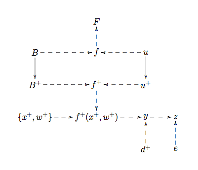
Figure 1: Bayesian belief network for Direct Reification.
Structural Reification
Structural Reification is a process where we link the current model \(f\) to an improved model \(f'\) , and then to the Reified model \(f^+\). Here \(f'\) may correspond to \(f_{\rm theory}\) or \(f'_{\rm theory}\) which were introduced in DiscReification.
Usually, we can think more carefully about the reasons for the model’s inadequacy. As we have advocated in the discussion page on expert assessment of model discrepancy (DiscExpertAssessMD), a useful strategy is to envisage specific improvements to the model, and to consider the possible effects on the model outputs of such improvements. Often we can imagine specific generalisations for \(f(x)\) with extra model components and new input parameters \(v\), resulting in an improved model \(f'(x, v)\) . Suppose the improved model reduces back to the current model for some value of \(v=v_0\) i.e. \(f'(x, v_0) = f(x)\) . We might emulate \(f'\) ‘on top’ of \(f\) , using the form:
where \(g_{ik}(x, v_0) = u^{(a)}_i(x, v_0) = 0\) . This would give the full emulator for \(f'_i(x, v)\) as
where for convenience we define \(B' = \{ \beta_{ij}, \gamma_{ik} \}\) and \(u' = u(x) + u^{(a)}(x,v)\). Assessment of the new regression coefficients \(\gamma_{ik}\) and stationary process \(u^{(a)}_i(x, v)\) would come from consideration of the specific improvements that \(f'\) incorporates. The reified emulator for \(f^+_i(x, v, w)\) would then be
where we would now carefully apportion the uncertainty between each of the random coefficients in the Reified emulator. Although this is a complex task, we would carry out this procedure when the expert’s knowledge about improvements to the model is detailed enough that it warrants inclusion in the analysis. An example of this procedure is given in Goldstein, M. and Rougier, J. C. (2009). We can represent this structure using the following Bayesian Belief Network, with \(B^+ = \{ \beta^+_{ij} , \gamma^+_{ik} \}\) , and \(u^+ = u^+(x)+u^+(x,v)+u^+(x,v,w)\):
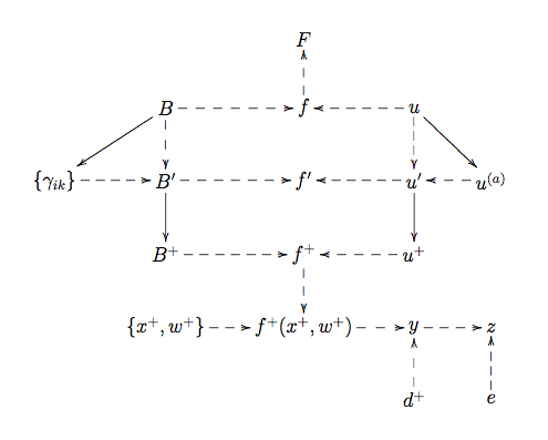
Figure 2: Bayesian belief network corresponding to Structured Reification.
Additional Comments
Once the emulator for \(f^+\) has been specified, the final step is to assess \(d^+\) which links the Reified model to reality. This is often a far simpler process than direct assessment of model discrepancy, as the structured beliefs about the difference between \(f\) and reality \(y\) have already been accounted for in the link between \(f\), \(f'\) and \(f^+\) . Reification also provides a natural framework for incorporating multiple models, by the judgement that each model will be informative about the Reified model, which is then informative about reality \(y\). Exchangeable Computer Models, as described in the discussion page DiscExchangeableModels, provide a further example of Reification. More details can be found in Goldstein, M. and Rougier, J. C. (2009).
References
Goldstein, M. and Rougier, J. C. (2009), “Reified Bayesian modelling and inference for physical systems (with Discussion)”, Journal of Statistical Planning and Inference, 139, 1221-1239.