Example: Using the Morris method
In the page we provide an example of applying the Morris screening method (ProcMorris) on a simple synthetic example.
Suppose the simulator function is deterministic and described by the formula \(f(x) = x_1 + x_2^2 + x_2 \times sin(x_3) + 0 \times x_4\). We will use the standard Morris method to discover the three relevant variables from a total set of four input variables.
We use \(R=4\) trajectories, four levels for each input \(p=4\) and \(\Delta=p/2(p-1) = 0.66\). Given these parameters, the total number of simulator runs is \((k+1)R = 20\). The experimental design used is shown below. The values have been rounded to two decimal places.
Morris Experimental Design
| \(x_1\) | \(x_2\) | \(x_3\) | \(x_4\) | \(f(x)\) |
|---|---|---|---|---|
| 0.00 | 0.33 | 0.33 | 0.00 | 0.22 |
| 0.67 | 0.33 | 0.33 | 0.00 | 0.89 |
| 0.67 | 1.00 | 0.33 | 0.00 | 1.99 |
| 0.67 | 1.00 | 0.33 | 0.67 | 1.99 |
| 0.67 | 1.00 | 1.00 | 0.67 | 2.51 |
| 0.33 | 0.00 | 0.33 | 0.33 | 0.33 |
| 0.33 | 0.00 | 1.00 | 0.33 | 0.33 |
| 1.00 | 0.00 | 1.00 | 0.33 | 1.00 |
| 1.00 | 0.67 | 1.00 | 0.33 | 2.01 |
| 1.00 | 0.67 | 1.00 | 1.00 | 2.01 |
| 0.00 | 0.00 | 0.00 | 0.33 | 0.00 |
| 0.00 | 0.00 | 0.67 | 0.33 | 0.00 |
| 0.67 | 0.00 | 0.67 | 0.33 | 0.67 |
| 0.67 | 0.67 | 0.67 | 0.33 | 1.52 |
| 0.67 | 0.67 | 0.67 | 1.00 | 1.52 |
| 0.33 | 0.33 | 0.00 | 0.00 | 0.44 |
| 0.33 | 0.33 | 0.67 | 0.00 | 0.65 |
| 1.00 | 0.33 | 0.67 | 0.00 | 1.32 |
| 1.00 | 0.33 | 0.67 | 0.67 | 1.32 |
| 1.00 | 1.00 | 0.67 | 0.67 | 2.62 |
Using this design we sampling statistics of the elementary effects for each factor are computed:
Morris Method Indexes
| Factor | \(\mu\) | \(\mu_*\) | \(\sigma\) |
|---|---|---|---|
| \(x_1\) | 1 | 1 | 2e-16 |
| \(x_2\) | 1.6 | 1.6 | 0.28 |
| \(x_3\) | 0.27 | 0.27 | 0.36 |
| \(x_4\) | 0 | 0 | 0 |
The \(\mu\) and \(\sigma\) values are plotted in Figure 1 below. As can be seen the Morris method effectively and clearly identifies the relevant inputs. For factor \(x_1\) we note the high \(\mu\) and low \(\sigma\) values signify a linear effect. For factors \(x_2\), \(x_3\) the large \(\sigma\) value demonstrates the non-linear/interaction effects. Factor \(x_4\) has zero value for both metrics as expected for an irrelevant factor. Lastly the agreement of \(\mu\) to \(\mu_*\) for all factors shows a lack of cancellation effects, due to the monotonic nature of the input-output response in this simple example. In general models this will not be the case, particularly those with non-linear responses.
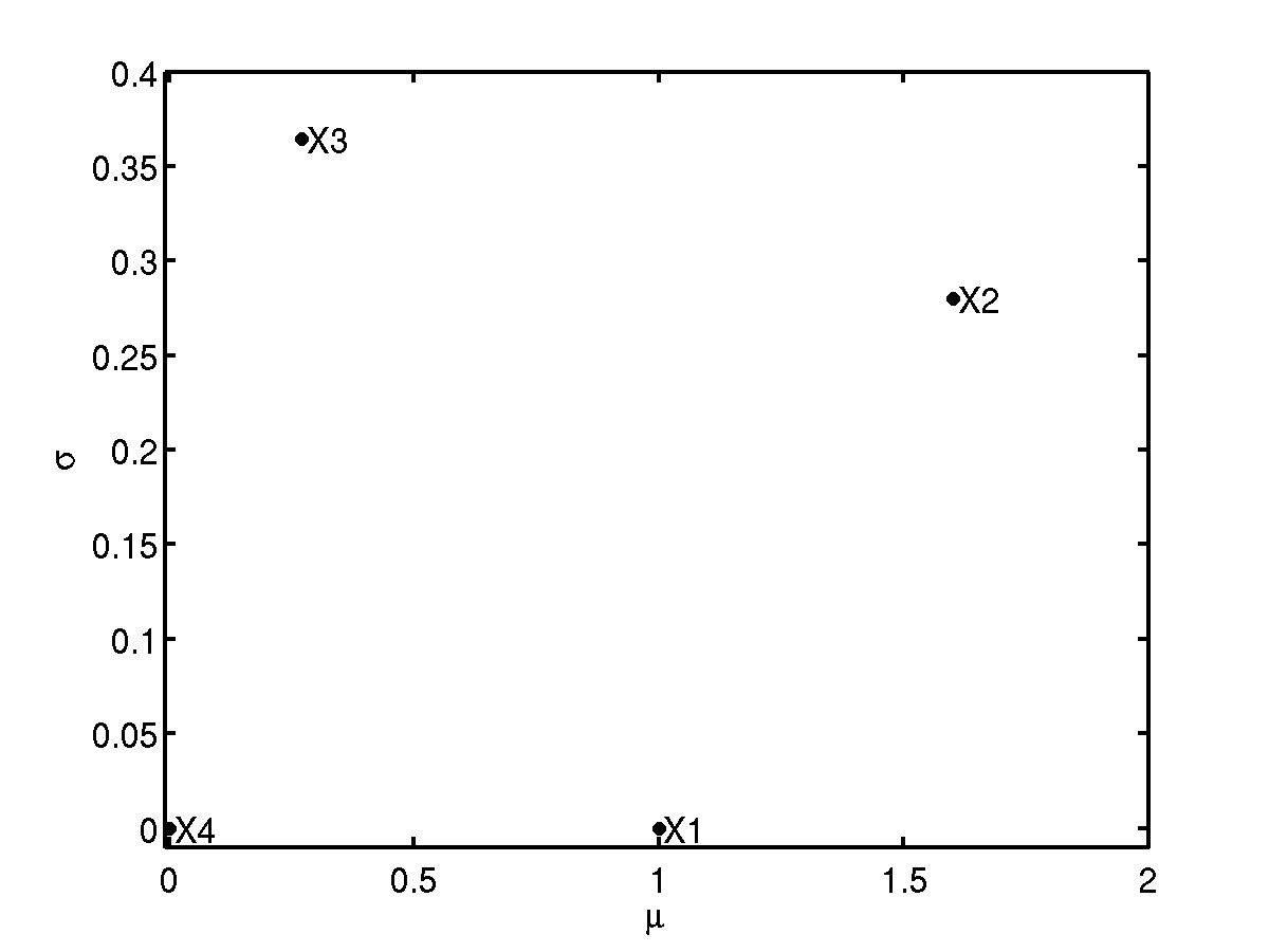
Figure 1: Summary statistics for Morris method.
References
A multitude of screening and sensitivity analysis methods including the Morris method are implemented in the sensitivity package available for the R statistical software system:
Gilles Pujol and Bertrand Iooss (2008). Sensitivity Analysis package: A collection of functions for factor screening and global sensitivity analysis of model output. http://cran.r-project.org/web/packages/sensitivity/index.html
R Development Core Team (2005). R: A language and environment for statistical computing. R Foundation for Statistical Computing, Vienna, Austria. ISBN 3-900051-07-0, http://www.R-project.org.