Example: A one dimensional emulator built with function output and derivatives
Simulator description
In this page we present an example of fitting an emulator to a \(p=1\) dimensional simulator when in addition to learning the function output of the simulator, we also learn the partial derivatives of the output w.r.t the input. The simulator we use is the function, \({\rm sin}(2x) + (\frac{x}{2})^2\). Although this is not a complex simulator which takes an appreciable amount of computing time to execute, it is still appropriate to use as an example. We restrict the range of the input, \(x\), to lie in \([-5,5]\) and the behaviour of our simulator over this range is shown in Figure 1. The simulator can be analytically differentiated to provide the relevant derivatives: \(2\cos(2x) + \frac{x}{2}\). For the purpose of this example we define the adjoint as the function which when executed returns both the simulator output and the derivative of the simulator output w.r.t the simulator input.
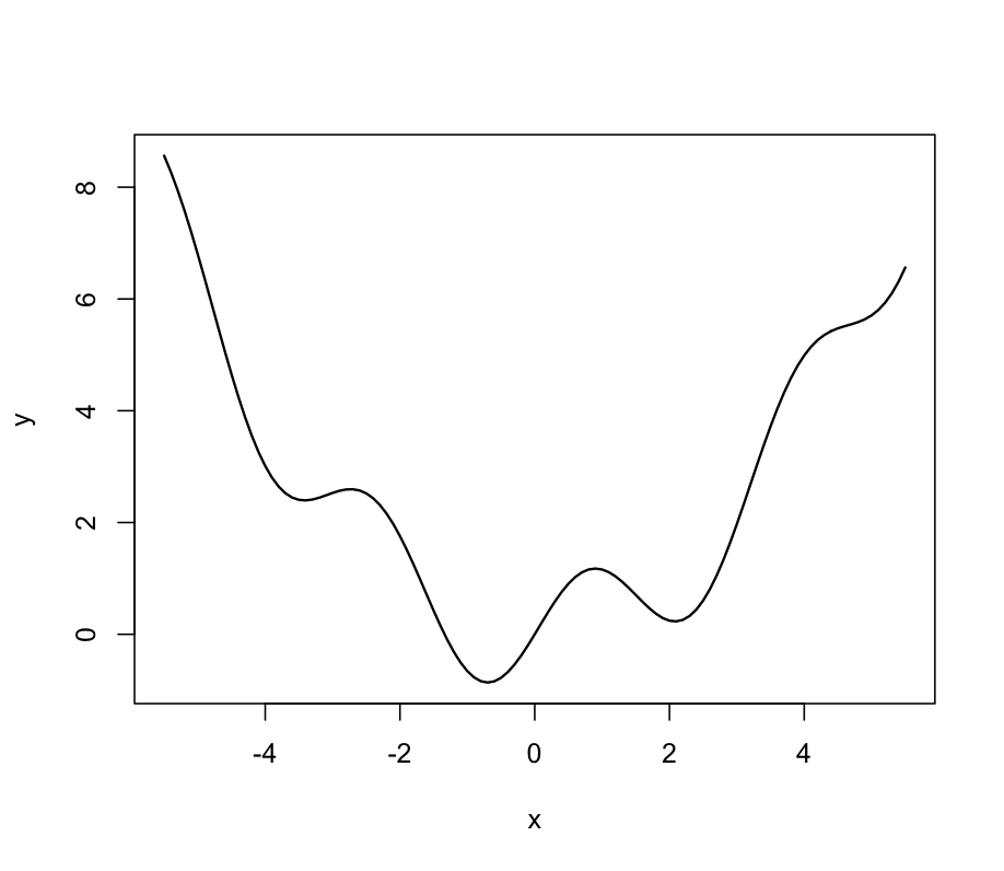
Figure 1: The simulator over the specified region
Design
We need to choose a design to select at which input points the simulator is to be run and at which points we want to include derivative information. An Optimised Latin Hypercube, which for one dimension is a set of equidistant points on the space of the input variable, is chosen. We select the following \(5\) design points:
We choose to evaluate the function output and the derivative at each of the \(5\) points and scale our design points to lie in \([0,1]\). This information is added to \(D\) resulting in the design, \(\tilde{D}\) of length \(\tilde{n}\). A point in \(\tilde{D}\) has the form \((x,d)\), where \(d\) denotes whether a derivative or the function output is to be included at that point; for example \((x,d)=(x,0)\) denotes the function output at point \(x\) and \((x,d)=(x,1)\) denotes the derivative w.r.t to the first input at point \(x\).
This results in the following design:
The output of the adjoint at these points, which make up our training data, is:
Note that the first \(5\) elements of \(\tilde{D}\), and therefore \(\tilde{f}(\tilde{D})\), are simply the same as in the core problem. Elements 6-10 correspond to the derivatives. Throughout this example \(n\) will refer to the number of distinct locations in the design (5), while \(\tilde{n}\) refers to the total amount of data points in the training sample. Since we include a derivative at all \(n\) points w.r.t to the \(p=1\) input, \(\tilde{n}=n(p+1)=10\).
Gaussian process setup
In setting up the Gaussian process, we need to define the mean and the covariance function. As we are including derivative information here we need to ensure that the mean function is once differentiable and the covariance function is twice differentiable. For the mean function, we choose the linear form described in the alternatives page on emulator prior mean function (AltMeanFunction), which is \(h(x) = [1,x]^{\rm T}\) and \(q=1+p = 2\). This corresponds to \(\strut \tilde{h}(x,0) = [1,x]^{\rm T}\) and we also have \(\frac{\partial}{\partial x}h(x) = [1]\) and so \(\tilde{h}(x,1) = [1]\).
For the covariance function we choose \(\sigma^2c(\cdot,\cdot),\) where the correlation function \(c(\cdot,\cdot)\) has the Gaussian form described in the alternatives page on emulator prior correlation function (AltCorrelationFunction). We can break this down into 3 cases, as described in the procedure page for building a GP emulator with derivative information (ProcBuildWithDerivsGP):
Case 1 is the correlation between points, so we have \(d_i=d_j=0\) and \(c\{(x_i,0),(x_j,0)\}=\exp\left[-\{(x_i - x_j)/\delta\}^2\right]\).
Case 2 is the correlation between a point, \(x_i\), and the derivatives at point \(x_j\), so we have \(d_i= 0\) and \(d_j\ne0\). Since in this example \(p=1\), this amounts to \(d_j=1\) and we have:
Case 3 is the correlation between two derivatives at points \(x_i\) and \(x_j\). Since in this example \(p=1\), the only relevant correlation here is when \(d_i=d_j=1\) (which corresponds to Case 3a in ProcBuildWithDerivsGP) and is given by:
Each Case provides sub-matrices of correlations and we arrange them as follows:
an \(\tilde{n}\times \tilde{n}\) matrix. The matrix \(\strut \tilde{A}\) is symmetric and within \(\tilde{A}\) we have symmetric sub-matrices, Case 1 and Case 3. Case 1 is an \(n \times n=5 \times 5\) matrix and is exactly the same as in the procedure page ProcBuildCoreGP. Since we are including the derivative at each of the 5 design points, Case 2 and 3 sub-matrices are also of size \(n \times n=5 \times 5\).
Estimation of the correlation length
We need to estimate the correlation length \(\delta\). In this example we will use the value of \(\delta\) that maximises the posterior distribution \(\pi^*_{\delta}(\delta)\), assuming that there is no prior information on \(\delta\), i.e. \(\pi(\delta)\propto \mathrm{const}\). The expression that needs to be maximised is (from ProcBuildWithDerivsGP)
where
We have \(\tilde{H}=[\tilde{h}(x_1,d_1),\ldots,\tilde{h}(x_{10},d_{10})]^{\rm T},\) where \(\tilde{h}(x,d)\) and \(\tilde{A}\) are defined above in section Gaussian process setup.
Recall that in the above expressions the only term that is a function of \(\delta\) is the correlation matrix \(\tilde{A}\).
The maximum can be obtained with any maximisation algorithm and in this example we used Nelder - Mead. The value of \(\delta\) which maximises the posterior is 0.183 and we will fix \(\delta\) at this value thus ignoring the uncertainty with it, as discussed in ProcBuildCoreGP. We refer to this value of \(\delta\) as \(\hat\delta\). We have scaled the input to lie in \([0,1]\) and so in terms of the original input scale, \(\hat\delta\) corresponds to a smoothness parameter of \(10\times 0.183 = 1.83\)
Estimates for the remaining parameters
The remaining parameters of the Gaussian process are \(\beta\) and \(\sigma^2\). We assume weak prior information on \(\beta\) and \(\sigma^2\) and so having estimated the correlation length, the estimate for \(\sigma^2\) is given by the equation above in section Estimation of the correlation length, and the estimate for \(\beta\) is
Note that in these equations, the matrix \(\tilde{A}\) is calculated using \(\hat{\delta}\). The application of the two equations for \(\hat\beta\) and \(\widehat\sigma^2\), gives us in this example \(\hat{\beta} = [ 4.734, -2.046]^{\rm T}\) and \(\widehat\sigma^2 = 15.47\)
Posterior mean and Covariance functions
The expressions for the posterior mean and covariance functions as given in ProcBuildWithDerivsGP are
and
Figure 2 shows the predictions of the emulator for 100 points uniformly spaced on the original scale. The solid, black line is the output of the simulator and the blue, dashed line is the emulator mean \(m^*\) evaluated at each of the 100 points. The blue dotted lines represent 2 times the standard deviation about the emulator mean, which is the square root of the diagonal of matrix \(v^*\). The black crosses show the location of the design points where we have evaluated the function output and the derivative to make up the training sample. The green circles show the location of the validation data which is discussed in the section below. We can see from Figure 2 that the emulator mean is very close to the true simulator output and the uncertainty decreases as we get closer the location of the design points.
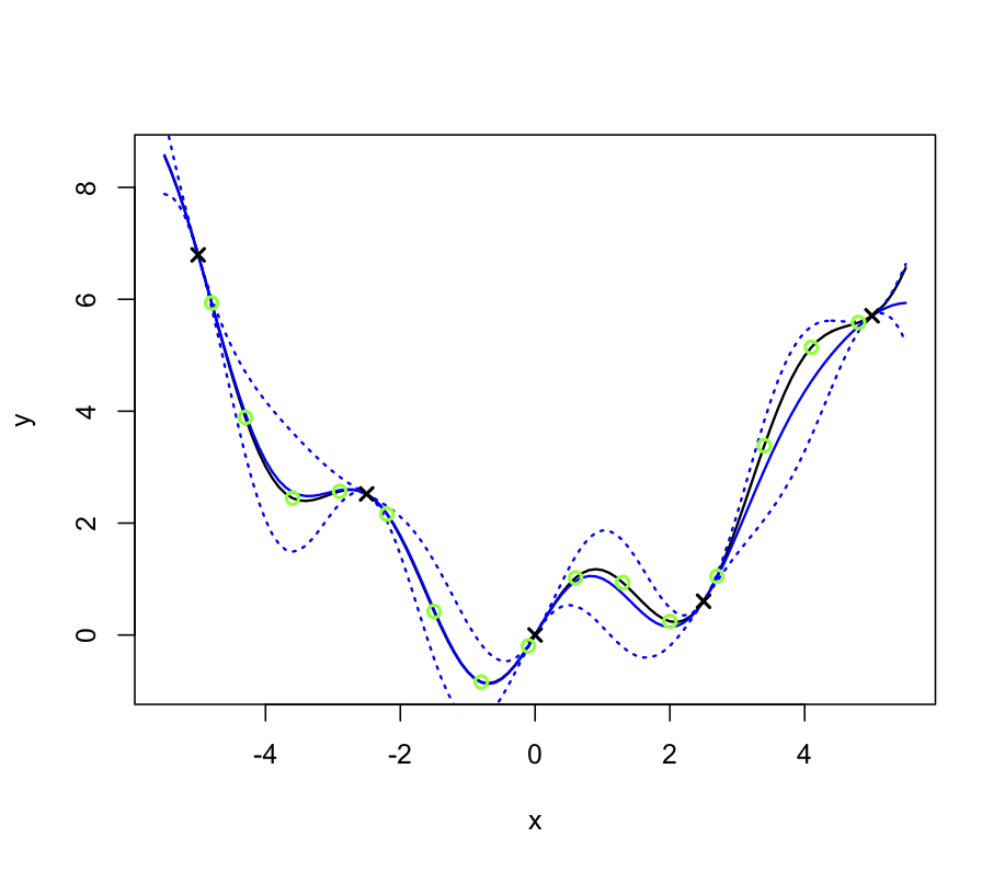
Figure 2: The simulator (solid black line), the emulator mean (blue, dotted) and 95% confidence intervals shown by the blue, dashed line. Black crosses are design points, green circles are validation points.
Validation
In this section we validate the above emulator according to the procedure page for validating a GP emulator (ProcValidateCoreGP).
The first step is to select the validation design. We choose here 15 space filling points ensuring these points are distinct from the design points. The validation points are shown by green circles in Figure 2 above and in the original input space of the simulator are:
and in the transformed space:
Note that the prime symbol \(^\prime\) does not denote a derivative, as in ProcValidateCoreGP we use the prime symbol to specify validation. We’re predicting function output in this example and so do not need validation derivatives; as such we have a validation design \(D^\prime\) and not \(\tilde{D}^\prime\). The function output of the simulator at these validation points is
We then calculate the mean \(m^*(\cdot)\) and variance \(v^*(\cdot,\cdot)\) of the emulator at each validation design point in \(D^\prime\) and the difference between the emulator mean and the simulator output at these points can be compared in Figure 2.
We also calculate standardised errors given in ProcValidateCoreGP as \(\frac{f(x^\prime_j)-m^*(x_j^\prime)}{\sqrt{v^*(x^\prime_j,x^\prime_j)}}\) and plot them in Figure 3.
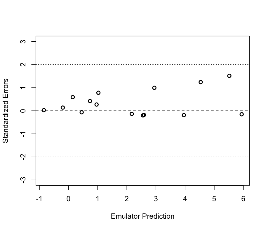
Figure 3: Individual standardised errors for the prediction at the validation points
Figure 3 shows that all the standardised errors lie between -2 and 2 providing no evidence of conflict between simulator and emulator.
We calculate the Mahalanobis distance as given in ProcValidateCoreGP:
when its theoretical mean is \({\rm E}[M] = n^\prime = 15\) and variance, \({\rm Var}[M] = \frac{2n^{\prime}(n^{\prime}+\tilde{n}-q-2)}{\tilde{n}-q-4} = 12.55^2\).
We have a slightly small value for the Mahalanobis distance therefore, but it is within one standard deviation of the theoretical mean. The validation sample is small and so we would only expect to detect large problems with this test. This is just an example and we would not expect a simulator of a real problem to only have one input, but with our example we can afford to run the simulator intensely over the specified input region. This allows us to assess the overall performance of the emulator and, as Figure 2 shows, the emulator can be declared as valid.
Comparison with an emulator built with function output alone
We now build an emulator for the same simulator with all the same assumptions, but this time leave out the derivative information to investigate the effect of the derivatives and compare the results.
We obtain the following estimates for the parameters:
Figure 4 shows the predictions of this emulator for 100 points uniformly spaced on the original scale. The solid, black line is the output of the simulator and the red, dashed line is the emulator mean evaluated at each of the 100 points. The red dotted lines represent 2 times the standard deviation about the emulator mean. The black crosses show the location of the design points where we have evaluated the function output. We can see from Figure 4 that the emulator is not capturing the behaviour of the simulator at all and further simulator runs are required.
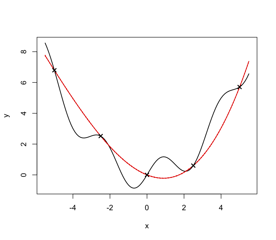
Figure 4: The simulator (solid black line), the emulator mean (red, dotted) and 95% confidence intervals shown by the red, dashed line. Black crosses are design points.
We add 4 further design points, \([-3.75, -1.25, 1.25, 3.75]\), and rebuild the emulator, without derivatives as before. This results in new estimates for the parameters, \(\hat\delta = 0.177, \hat{\beta} = [ 4.32, -2.07]^{\rm T}\) and \(\widehat\sigma^2 = 15.44\), and Figure 5 shows the predictions of this emulator for the same 100 points. We now see that the emulator mean closely matches the simulator output across the specified range.
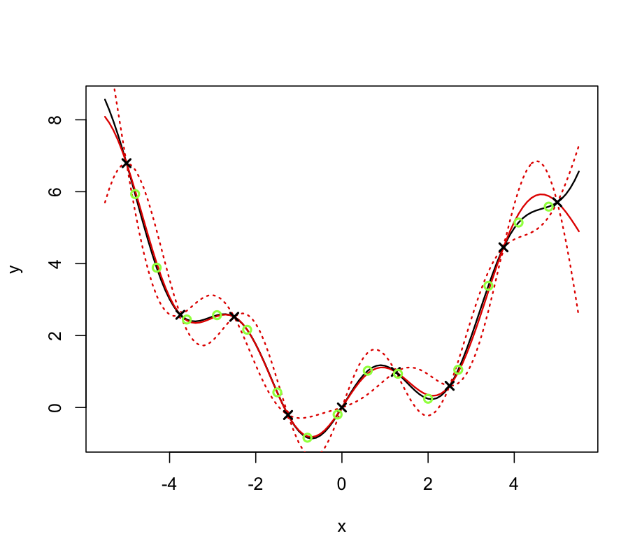
Figure 5: The simulator (solid black line), the emulator mean (red, dotted) and 95% confidence intervals shown by the red, dashed line. Black crosses are design points, green circles are validation points.
We repeat the validation diagnostics using the same validation data and obtain a Mahalanobis distance of 4.70, while the theoretical mean is 15 with standard deviation 14.14. As for the emulator with derivatives, a value of 4.70 is bit small; however the standardised errors calculated as before, and shown in Figure 6 below, provide no evidence of conflict between simulator and emulator and the overall performance of the emulator as illustrated in Figure 5 is satisfactory.
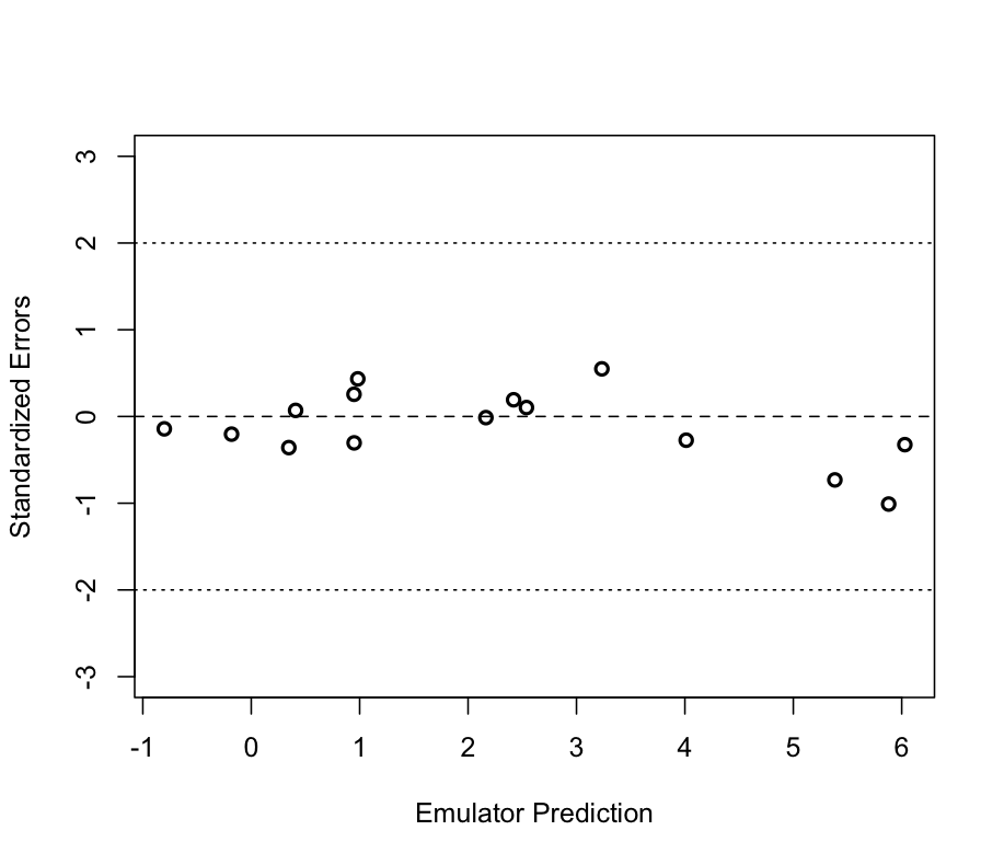
Figure 6: Individual standardised errors for the prediction at the validation points
We have therefore now built a valid emulator without derivatives but required 4 extra simulator runs to the emulator with derivatives, to achieve this.